Intermediate
Macroeconomics

Lecture 6

Consumption and Savings

In This Lecture

• How to think about consumer savings in a model
• Effect of changes in interest rate
• Effect of changes in present or future income

Consumption Savings Model

• Consider a model with only two periods: today and tomorrow
• Consumers have a certain income today ($y$), income tomorrow ($y^{\prime}$), taxes today ($t$), and taxes tomorrow ($t^{\prime}$)
• They must choose an amount to save ($s$), as well as consumption today ($c$) and consumption tomorrow ($c^{\prime}$)

Budget Constraint(s)

• Now we have two budget constraints, one for each period. Today
$$c + s = y - t$$
• And for tomorrow
$$c^{\prime} = y^{\prime} - t^{\prime} + (1+r) s$$
• Notice that saving yields a return of $1+r$, the interest rate

Moving to One Constraint

• In first period, anything you don't consume, you must save
$$s = (y - t) - c$$
• Plugging this into second period budget constraint
$$c^{\prime} = y^{\prime} - t^{\prime} + (1+r)(y - t - c)$$
• So now we have one budget constraint relating consumption today and consumption tomorrow

Lifetime Budget Constraint

• We can express this as a lifetime budget constraint
$$\begin{align*} & c^{\prime} = y^{\prime} - t^{\prime} + (1+r)(y - t - c) \\ \Rightarrow\ & c + \frac{c^{\prime}}{1+r} = y - t + \frac{y^{\prime}-t^{\prime}}{1+r} \equiv we \longleftarrow \text{wealth} \end{align*}$$
• This says that the present value of your consumption is equal to the present value of your after-tax income (your wealth)
• This same as Walrasian model with $p = 1$ and $p^{\prime} = \frac{1}{1+r}$

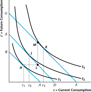
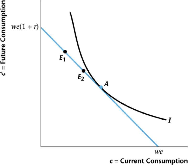
Visualizing Consumer Choices

Two "goods" are consumption today and tomorrow

Conditions for Optimality

• Remember the Walrasian model said the optimum should equate the marginal rate of substitution with the price ratio
• Here that means the interest rate, so that
$$\text{MRS}_{c,c^{\prime}} = 1 +r$$
• Give $1$ unit of consumption today $\rightarrow$ get $1+r$ units tomorrow
• This conditions means doing so wouldn't make you better or worse off

Consumption Smoothing

Consumers prefer to smooth consumption across periods

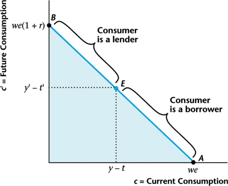
Borrowers and Lenders

Final consumption only depends on present value wealth.
Split between today and tomorrow — lender or borrower.

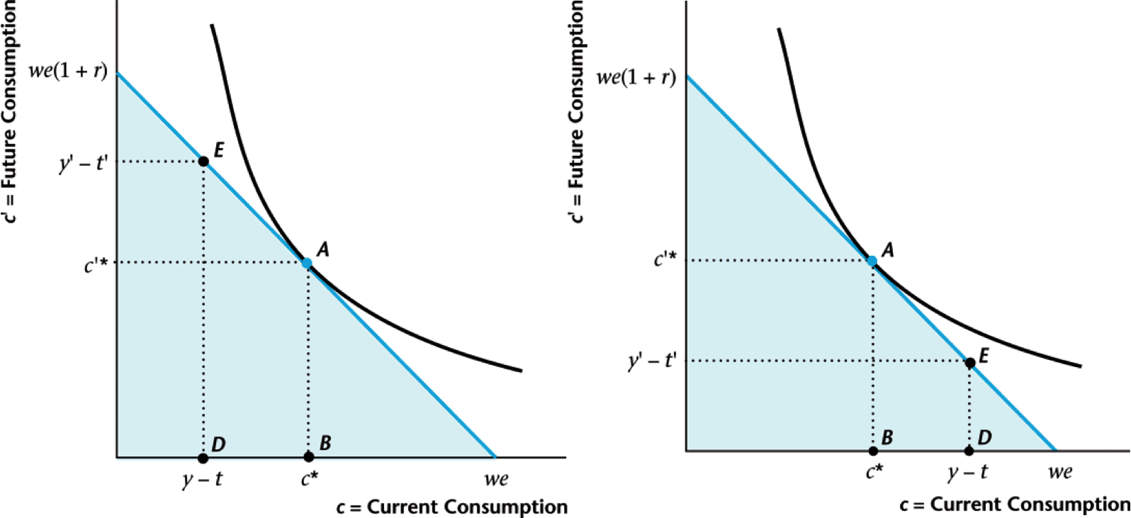
Increase in Current Income

What happens when your income today increases?

Permanent Income

• Your present day consumption increases by less than income increase
• Increase "unbalances" your income, so you save a bit more to smooth consumption
• The same thing is true of increases in future income: future consumption goes up but
• You will also save slightly less and consume more today

Increase in Future Income

What to do today if you got a nice job starting next year?

Time Series Implications

• Given what we have found, we would expect consumption to be smooth in the data
$$\text{Income} = \text{Consumption} + \text{Savings}$$
• If we smooth consumption, then we must do so by adjusting savings, making it more volatile
$$Vol(\text{Consumption}) < Vol(\text{Income}) < Vol(\text{Savings})$$

Types of Consumption

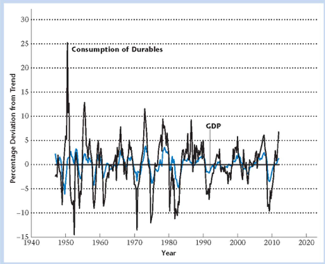
• Instead of savings, we can look at consumption of durables, which are things like cars and appliances
• These will act kind of like savings, since you give up current consumption to buy an appliance today for a future stream of consumption (household services)
• We will call regular consumption like food non-durables

Volatility of Consumption

Durables much more volatile than income (GDP)

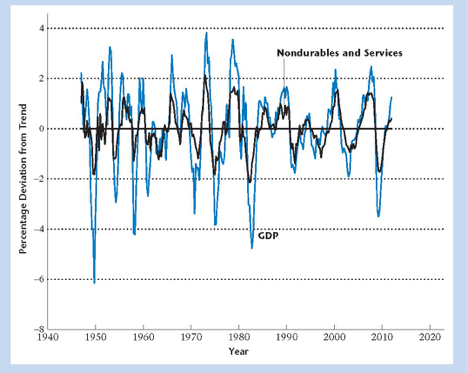
Volatility of Consumption

Non-durables much smoother than income (GDP)

Temporary vs Permanent

Temporary — current income $\uparrow$, permanent — both $\uparrow$

Consumption-Savings Response

• During 2008 recession, policymakers wanted to increase demand
• Giving people money (temporary stimulus) might just result in increased savings
• Efforts were made to target those most likely to spend (due to borrowing limits)
• We'll talk later about the broader issues involved

Permanent Changes in Wealth

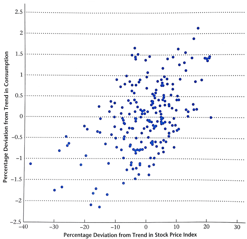
Movements in stock prices are correlated with non-durables

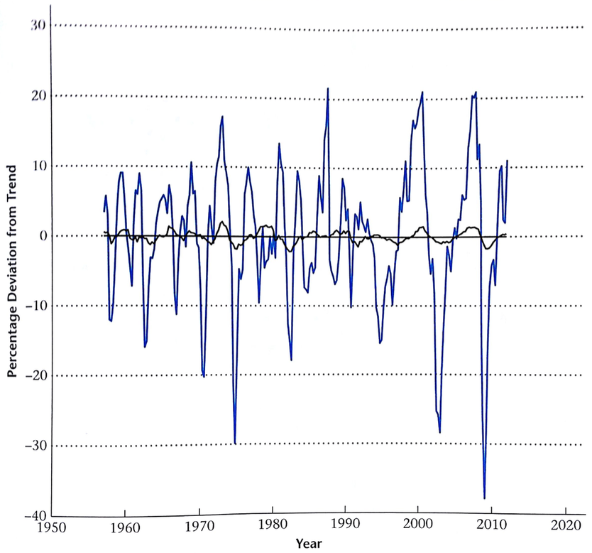
Permanent Changes in Wealth

Theory says movements in stocks should be "permanent"

Interest Rate Response

• How might a consumer respond to changes in the interest rate?
• This is slightly more nuanced the the income case
• Interest rate changes both wealth (present value of income) and prices
• So we have an income and substitution effect

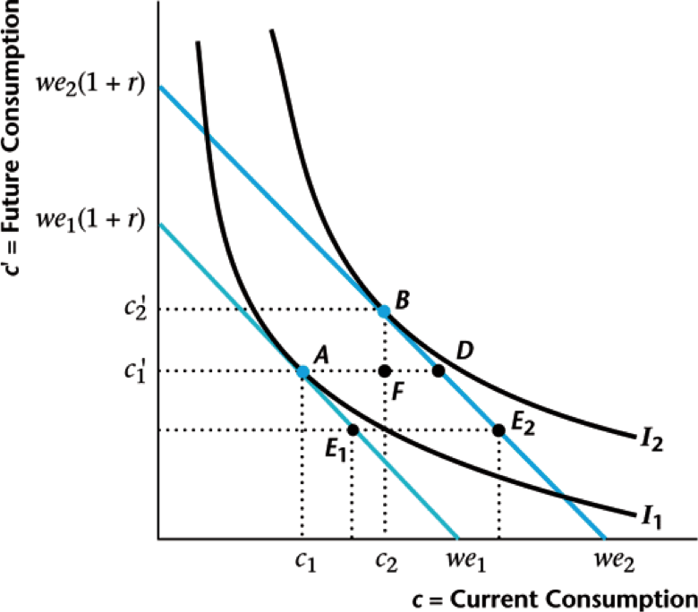
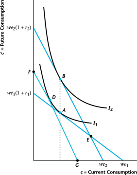
Effect On Savers

Substitution effect: $A \rightarrow D$ ($r \uparrow$ so more savings)
Income effect: $D \rightarrow B$ (income $\uparrow$ so more of both)

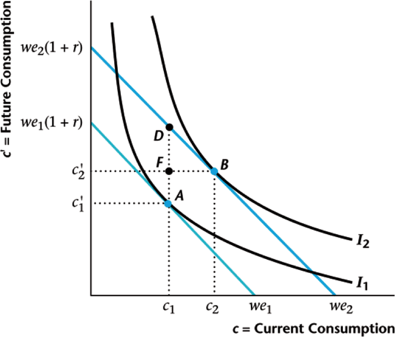
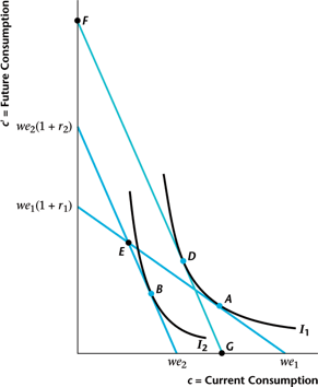
Effect On Borrowers

Substitution effect: $A \rightarrow D$ ($r \uparrow$ so more savings)
Income effect: $D \rightarrow B$ (income $\downarrow$ so less of both)

Breaking Down Effects

• If interest rate goes up, doesn't wealth go down? Yes!
• Price variation uses Hicksian demand at old utility and new prices (min cost subject to utility unchanged)
• Moving from price modified demand to final demand?
• Residual income change depends on whether you started as saver or borrower

Savers Vs Borrowers

Summary Of Effects

• Savers
  • Future consumption increases
  • Current consumption/savings may rise or fall
• Borrowers
  • Current consumtion falls (savings increases)
  • Future consumption may rise or fall

Theoretical Underpinnings

• Suppose our consumer has utility of the form
$$U(c,c^{\prime}) = u(c) + \beta u(c^{\prime})$$
• Little $u$ is called the per-period or Bernoulli utility function
• Utility of this form is called separable
• The weight $\beta$ on the second period is called the discount rate

Intertemporal Optimization

• The problem the consumer solves is
$$\begin{align*} \max_{c,c^{\prime}} \quad & u(c) + \beta u(c^{\prime}) \\ s.t \quad & c + \frac{c^{\prime}}{1+r} = y-t + \frac{y^{\prime}-t^{\prime}}{1+r} = we \end{align*}$$
• We can also think about his as just choosing the savings $s$
$$\max_{s} \quad u(y-t-s) + \beta u(y^{\prime}-t^{\prime}+(1+r)s)$$
• These will always give the same answer in the end!

Optimal Savings Choice

• Let's go with the savings choice and take the derivative with respect to $s$
$$\begin{align*} & 0 = -u_c(y-t-s) + \beta (1+r) u_c (y^{\prime}-t^{\prime}+(1+r)s) \\ \Rightarrow\ & u_c(c) = \beta (1+r) u_c(c^{\prime}) \\ \Rightarrow\ & \frac{u_c(c)}{u_c(c^{\prime})} = \beta (1+r) \qquad \Leftrightarrow \quad MRS = \frac{u_c(c)}{\beta u_c(c^{\prime})} = 1+r \end{align*}$$
• This is the same MRS condition I mentioned earlier and that we see in the graphs

Consumption Smoothing

• That first condition is also called the Euler condition
$$\frac{u_c(c)}{u_c(c^{\prime})} = \beta (1+r)$$
• Remember that the function $u_c(\cdot)$ is just marginal utility
• We assume that this is decreasing, so its a monotone function
• What happens when $\beta (1+r) = 1$?
$$\beta(1+r) = 1 \quad \Rightarrow \quad u_c(c) = u_c(c^{\prime}) \quad \Rightarrow \quad c = c^{\prime}$$

Consumption Smoothing

• So when $1+r = 1/\beta$, we get perfect consumption smoothing
• You can also show that when $1+r \ge 1/\beta$, you get $c < c^{\prime}$ and vice versa
• Makes sense: high interest rate $\rightarrow$ people save more
• Turns out this isn't too unreasonable, often $r$ is around $0.05$ and we usually use $\beta = 0.95$
$$(1+0.05) \times 0.95 \approx 1$$

A Specific Example

• Now let's specify a functional form for $u(\cdot)$ with
$$u(c) = \log(c)$$
• Thus our utility function, fully fledged, is given by
$$u(c,c^{\prime}) = \log(c) + \beta \log(c^{\prime})$$
• The Euler/MRS condition tells us the ratio of future to present consumption
$$1+g = \frac{c^{\prime}}{c} = \beta(1+r)$$

A Specific Example

• What about the exact levels of $c$ and $c^{\prime}$?
• We can get those from the budget constraint and the Euler equation combined
$$c = \left(\frac{1}{1+\beta}\right) we \qquad c^{\prime} = \left(\frac{\beta(1+r)}{1+\beta}\right) we$$
• Can also calculate savings $s = y - t - c$
$$s = \left(\frac{\beta}{1+\beta}\right) \left[y-t - \frac{y^{\prime}-t^{\prime}}{\beta(1+r)}\right]$$

Savings in the Data

Fairly large dispersion around 20% savings rate

Introducing a Government

• Let's think about the role of government now
• In US, federal government buys and sells bonds to affect interest rates
• Does so through the semi-independent Federal Reserve system
• Similar systems in place throughout most of the world

Historical Interest Rates

This shows the Federal Funds Rate since 1954

Government Budget

• Suppose we have a unitary government that
  • Levies taxes $T$ and $T^{\prime}$
  • Has spending levels $G$ and $G^{\prime}$
  • Sells bonds $B$ to people at rate $r$
• This leads to present and future budget constraints
$$\begin{align*} & G = T + B \\ & G^{\prime} + (1+r) B = T^{\prime} \end{align*}$$

Government Present Value

• Now lets combine these two as we did with the consumers'
$$\begin{align*} & G^{\prime} + (1+r) (G-T) = T^{\prime} \\ \Rightarrow\ & G + \frac{G^{\prime}}{1+r} = T + \frac{T^{\prime}}{1+r} \end{align*}$$
• Just as before, the present value of government spending equals present value of government taxation

Connecting With Consumer

• When there $N$ consumers in the economy, the total tax amounts satisfy
$$T = t N$$
• Thus we can calculate the present value of each person's taxes
$$\begin{align*} & T + \frac{T^{\prime}}{1+r} = G + \frac{G^{\prime}}{1+r} \\ \Rightarrow\ & t + \frac{t^{\prime}}{1+r} = \frac{1}{N}\left[G + \frac{G^{\prime}}{1+r}\right] \end{align*}$$

Ricardian Equivalence

• In the consumer's budget equation we get
$$c + \frac{c^{\prime}}{1+r} = y + \frac{y^{\prime}}{1+r} - \frac{1}{N}\left[G + \frac{G^{\prime}}{1+r}\right]$$
• Thus the timing over government spending/taxes doesn't matter, only the present value does
• This notion is called Ricardian equivalence
• No change if the government reduced taxes today by $\$100$ and increased taxes tomorrow by $(1+r) \times \$100$ tomorrow (using $\$100$ increase in bonds $B$)

Consumer Response

Consumer will simply save extra after tax income: no change

Assumptions Invoked Here

• Tax changes are the same for all consumers in both present and future (no redistribution)
• Debt issued by the government is paid off during the lifetimes of the people alive when the debt was issued
• Taxes are "lump sum" rather than proportional (like income tax)
• Consumers and government face same interest rate and are free to borrow and lend

Real-world Example

• Does this apply to Bush tax cuts of 2001 (aka EGTRRA)?
• Reduced marginal income tax rates (graduated scheme)
• Credit constraints: went mostly to high earners, so not a big issue
• Taxes are proportional, not lump-sum, so they could be distortionary (reduce incentive to work)
• What will happen to future spending/taxation? People might expect lower spending in future

Government Debt Dynamics

• What happens when government runs consistent deficits?
$$\text{(Surplus)} \quad S = T - G$$
• Suppose that government runs a fixed surplus in each period
$$S_t = a Y_t = a (1+g)^t Y_0$$
• Surplus $a$ can be positive or negative (deficit), constant economic growth rate $g$

Debt Flows and Stocks

• Government debt is the accumulation of deficits over time
• Let the debt level be $D_t$ so that
$$D_t = (1+r)D_{t-1} - S_t = (1+r)D_{t-1} - a Y_t$$
• We want to think about the debt/GDP ratio $d_t = D_t/Y_t$
$$\begin{align*} & \frac{D_t}{Y_t} = (1+r)\frac{D_{t-1}}{Y_t} - a = (1+r)\frac{D_{t-1}}{Y_{t-1}}\frac{Y_{t-1}}{Y_t} - a \\ \Rightarrow\ & d_t = \left(\frac{1+r}{1+g}\right) d_{t-1} - a \end{align*}$$

Convergence of Debt/GDP

• Does this process converge? Use techniques we saw with capital growth ($k_t = k_{t-1} = k^{\ast}$)
• Suppose we always runs a deficit so that $a \lt 0$
• Then we need $r \lt g$ to converge!
$$\begin{align*} & d_t = \left(\frac{1+r}{1+g}\right) d_{t-1} - a \\ \Rightarrow\ & d^{\ast} = \left(\frac{1+r}{1+g}\right) d^{\ast} - a = \frac{-a(1+g)}{g-r} \end{align*}$$

Does It Converge?

• There are actually some reasons to think that $r \gt g$
• Right now $r \lt g$, but this has often not been the case
• From theory we saw earlier
$$1+g = \beta (1+r) \quad \Rightarrow \quad r \gt g$$
• In fact, the most concise three character summary of Piketty's recent Capital in the 21st Century is simply $$"r \gt g"$$

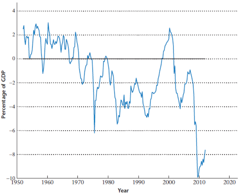
Government Surplus Data

This is what it looks like for the US since 1950

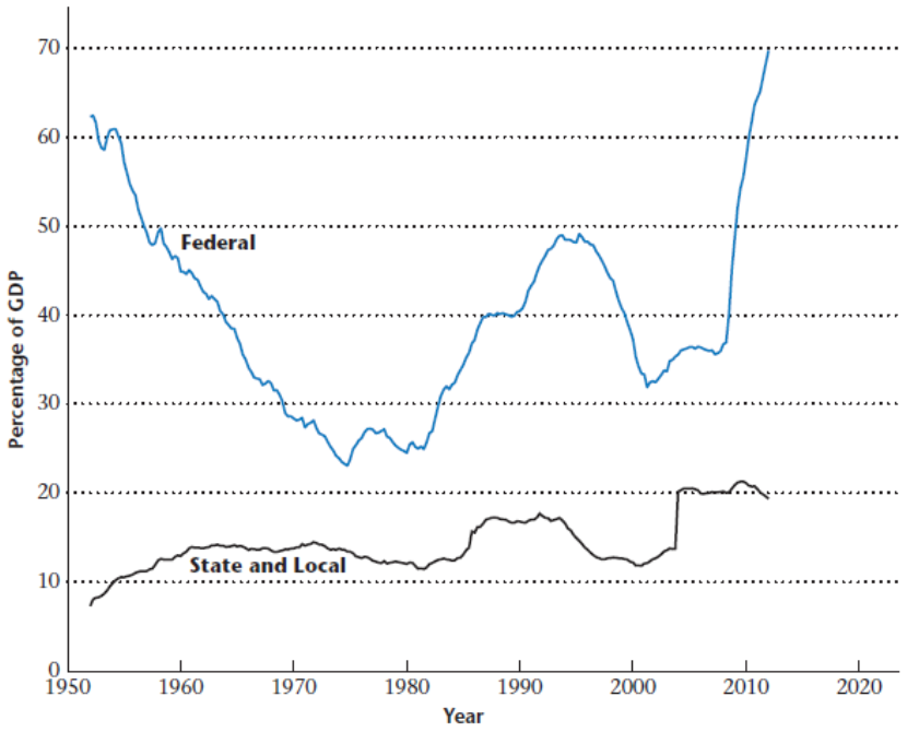
Government Debt Data

This is what we see in the US since 1950

Aggregate Assumptions

• Suppose the primary deficit (the deficit minus interest payments on the government debt) is a constant fraction of GDP forever.
• Real GDP grows at its average rate, 3% per year, forever.
• The real interest rate is 2% per year, forever.

Steady State Calculations

• Primary deficit of 5% of GDP forever implies: Debt/GDP ratio of 515% in the long run, with 10.3% of GDP spent on interest payments on the government debt per year in the long run.
• Primary deficit of 2.5% of GDP forever implies: Debt/GDP ratio of 258% in the long run, with 5.2% of GDP spent on interest payments on the government debt.

Cross Country Data

Here we have central government debt for OECD countries