Intermediate
Macroeconomics
Extra Lecture
Douglas Hanley, University of PittsburghEconomics of Ideas
In This Lecture
- Up until now, we've looked at economies without technological growth or with exogenous technological change
- We've also looked across countries to figure out differences in TFP and TFP growth
- But what drives technological growth in frontier economies such as the US?
Properties of Ideas
- Ideas or “knowledge capital” are different from other forms of capital because they are non-rivalrous
- I can employ a certain method or technology independent of whether you do — not true for physical capital
- They are also often non-excludable: it is difficult for me to prevent you from utilizing a particular technology
Types of Goods
Using these two binary distinctions, we can classify goods into four basic categories
$$ \begin{array}{l|c|c} & \textbf{Rivalrous} & \textbf{Non-rivalrous} \\ \hline \textbf{Excludable} & \text{Physical goods} & \text{DRM content} \\ \hline \textbf{Non-excludable} & \text{GM seeds} & \text{Basic science} \\ \end{array} $$Increasing Returns
- Non-rivalrous goods are inherently linked to the notion of increasing returns to scale
- Producing a piece of software generally requires a single up-front investment — distributing said software, particularly nowadays, is relatively costless
- Cost-per-user decreases with number of users $\longrightarrow$ increasing returns
Market Size Effects
- Markets with more potential users/consumers should attract more innovators
- Example — look at number of apps on iPhone, Android, Windows Phone (1.4M, 1.5M, 300K)
- Can we apply this logic to world population? — more population $\rightarrow$ more innovation
Scale Effects
- Such dependence of economic growth on population size is called a scale effect
- We don't see evidence of this dynamic at the country level (or language level) or globally over time
- What we do see is that economic growth moves with population growth — but which causes which?
Population Growth
Historic population growth rates from Jones (2002)

(Im)perfect Competition
- In software story before, we had large fixed cost but near zero marginal cost of production
- A competitive market would result in a price of zero — then what firm would want to pay up front cost?
- To get around this, innovating firms are granted temporary monopolies on their ideas called patents
Patent System
- England's Statute of Monopolies (1624) was first instance of something like a patent law
- The Crown had been granting monopolies on goods before this — this was the first to restrict usage to novel products
- Creating legal institutions to determine what is and is not novel was (and still is) quite difficult
Patent Policy
- Fundamental tradeoff of patent policy is that one wants to encourage innovation, but monopolies introduce product market distortions (micro)
- Long-lasting patents will spur innovation but have large monopoly distortions — short patents just the opposite
- The US Patent Office uses a 20-year patent length, as do most other countries
Patent History
Patenting has risen dramatically since 1980

Scientists and Engineers
Number of researchers has also risen dramatically

Growth in Output
Inputs have grown, but what about outputs?

A Soloesque Model
- We see that the inputs to innovation are growing (patents R&D), but outputs (productivity growth) are not
- It must be that innovation is getting more difficult as time and technology progress
- Let's build a model to incorporate this notion into the process of economic growth through innovation
Romer Model
- This will build off of a seminal paper by Paul Romer in 1990 entitled “Endogenous Technological Change”
- Here technology will be denoted by $A$ instead of $z$ and will enter into production in a slightly different way $$Y = K^{\alpha} (AL_P)^{1-\alpha}$$
- When technology is attached to labor rather than going out front, it is called labor-augmenting
Capital and Labor
- Our inputs will move around much the same way they did in the Solow model
- Capital will accumulate through the net effect of a savings rate $s_K$ and a depreciation rate $d$ $$K^{\prime} = s_K Y + (1-d) K$$
- Labor will grow at a constant rate $n$ $$L^{\prime} - L = n L$$
Technological Growth
- The rate of change of technology $A$ will be a function of research labor $L_A$ and the current technology level $A$ $$A^{\prime} - A = \delta L_R^{\lambda} A^{\phi}$$
- The parameter $\lambda \lt 1$ represents decreasing returns to scale in research, while $\phi$ represents how research difficulty depends on the technology level
- When $\phi \lt 1$, research gets more and more difficult as technology advances (seems intuitive)
Investment Decisions
- Now there is investment in both capital and technology growth, both of which we take as exogenous
- The capital investment rate $s_K$ works the same as it did in the standard Solow model
- The technology investment parameter is $s_R$, the fraction of labor devoted to research $$L_R = s_R L \quad \text{and} \quad L_P = (1-s_R) L$$
Short-run Growth Rate
- At any given time, we can calculate the growth rate of technology $$g_A = \frac{A^{\prime}-A}{A} = \frac{\delta L_R^{\lambda}}{A^{1-\phi}} = \delta s_R^{\lambda} \cdot \frac{L^{\lambda}}{A^{1-\phi}}$$
- In general this growth rate can be changing over time as well, but we expect it to settle down at some point
Long-run Growth Rate
- When the growth rate itself is constant over time we have $$\begin{align*} g^{\prime}_A &= g_A \\ \delta s_R^{\lambda} \cdot \frac{(L^{\prime})^{\lambda}}{(A^{\prime})^{1-\phi}} &= \delta s_R^{\lambda} \cdot \frac{L^{\lambda}}{A^{1-\phi}} \\ \left(\frac{L^{\prime}}{L}\right)^{\lambda} &= \left(\frac{A^{\prime}}{A}\right)^{1-\phi} \\ (1+n)^{\lambda} &= (1+g_A)^{1-\phi} \end{align*}$$
Long-run Growth Rate
- Solving for $g_A$ we can then find the long-run growth rate $$\begin{align*} & 1+g_A^{\ast} = (1+n)^{\frac{\lambda}{1-\phi}} \\ \Rightarrow\ & g_A^{\ast} \approx \frac{\lambda n}{1-\phi} \end{align*}$$
- Notice that the long-run growth rate is only a function of population growth $n$ and technology parameters $\lambda$ and $\phi$
- Somewhat surprising that amount of research $s_R$ does not affect long-run growth!
Comparative Statics
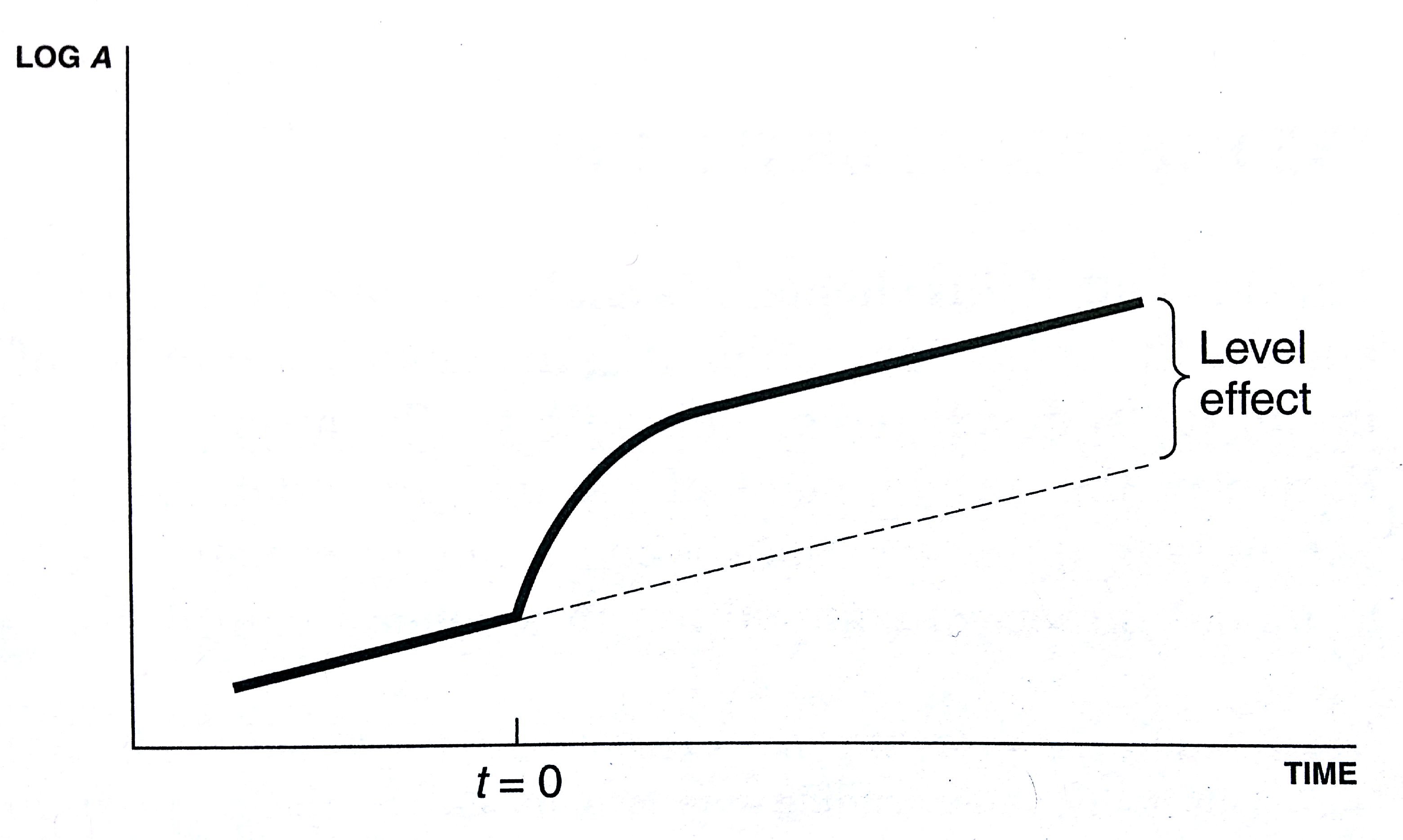
- What happens is we do increase $s_R$? Perhaps through an R&D subsidy
- Initially, the growth rate $g_A$ will jump up — over time this will make $A$ increase at a faster rate
- This makes R&D in the future even more difficult — eventually this will push the growth rate back down to the long-run value $g_A^{\ast}$
Short-run Dynamics
Growth rate and output dynamics with positive shock
 |
 |