Intermediate
Macroeconomics

Lecture 8

Savings and Investment

In This Lecture

• With the Solow model, we took the capital investment rate $s$ as given
• In the previous chapter we studied savings decisions by consumers
• Now we'll be these two together: consumers will save and this savings will go towards capital investment by firms
• We call this a “real” intertemporal model of savings and investment

Why a “Real” Model?

• Recall the distinction between real and nominal quantities
• Real quantities denote physical amounts of goods or inflation adjusted monetary values
• Nominal quantities are in pure monetary terms: changes in the value of money also change all nominal quantities
• In this model, there is no money. When you put savings in the bank, the interest rate tells you exactly how much you'll have next period and how much you can buy with it.

Elements of the Model

• There are two periods: we'll talk about today (plain) and tomorrow (with a prime: $\prime$)
• Consumers: make consumption/savings and labor/leisure decisions
• Firms: hires labor, makes investment, produces goods
• Government: spends, taxes, and borrows

Putting Things Together

• We can write a single pair of budget constraints to capture everything
$$\begin{align*} c + s &= w h + \pi - T \\ c^{\prime} &= w^{\prime} h^{\prime} + (1+r) s + \pi^{\prime} - T^{\prime} \end{align*}$$
• Combining these into a present value budget constraint
$$c + \frac{c^{\prime}}{1+r} = w h + \pi - T + \frac{w^{\prime}h^{\prime}+\pi^{\prime}-T^{\prime}}{1+r}$$

Labor-Lesiure Tradeoff

• Instead of going through everything again, we're going to use what we found in previous lectures
• The consumer is trading off the extra consumption from working more with the associated reduction in leisure
• We found that at the optimum, the consumer equates the MRS between consumption and leisure with the wage
$$MRS_{\ell,c} = w \qquad \qquad MRS_{\ell^{\prime},c^{\prime}} = w^{\prime}$$

Consumption-Savings Tradeoff

• At the same time, consumers are trading off consumption today and tomorrow
• They will choose to save or borrow until their Euler condition is satisfied, which we found to be
$$MRS_{c,c^{\prime}} = 1+r$$

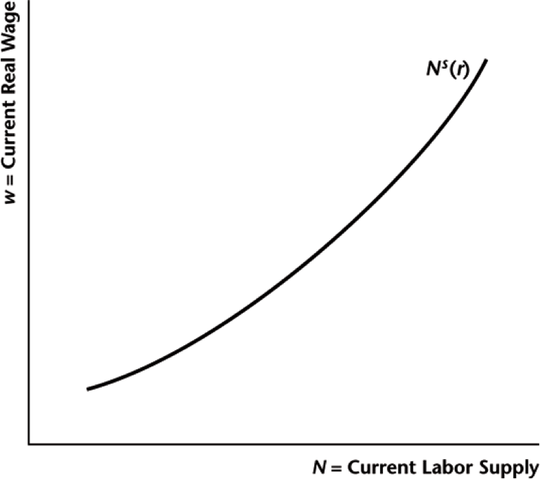
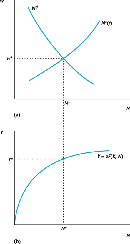
Aggregate Labor Supply

Higher wage rate $\rightarrow$ more labor supplied

Leisure Smoothing?

• Remember MRS's are just ratios of marginal utilities, so that
$$MRS_{\ell,\ell^{\prime}} = \frac{u_{\ell}/u_c}{u_{\ell^{\prime}}/u_{c^{\prime}}} \cdot \frac{u_c}{u_{c^{\prime}}} = \frac{MRS_{\ell,c}}{MRS_{\ell^{\prime},c^{\prime}}} \cdot MRS_{c,c^{\prime}} = \frac{w}{w^{\prime}} \cdot (1+r)$$
• With logarithmic utility, $u_{\ell} = 1/\ell$ and $u_{\ell^{\prime}} = 1/\ell^{\prime}$ so that
$$\frac{\ell^{\prime}}{\ell} = \frac{w}{w^{\prime}} \cdot \beta (1+r)$$
• So when the interest rate goes up, you consume more leisure tomorrow relative to today (work today to take advantage of high return on savings)

Labor and the Interest Rate

• We see "leisure smoothing" with the consumer
$$\frac{\ell^{\prime}}{\ell} = \frac{w}{w^{\prime}} \cdot \beta (1+r)$$
• A higher interest rate will lead to more leisure tomorrow relative to today
• This means more working today relative to tomorrow: the consumer works more so they can take advantage of higher savings rate

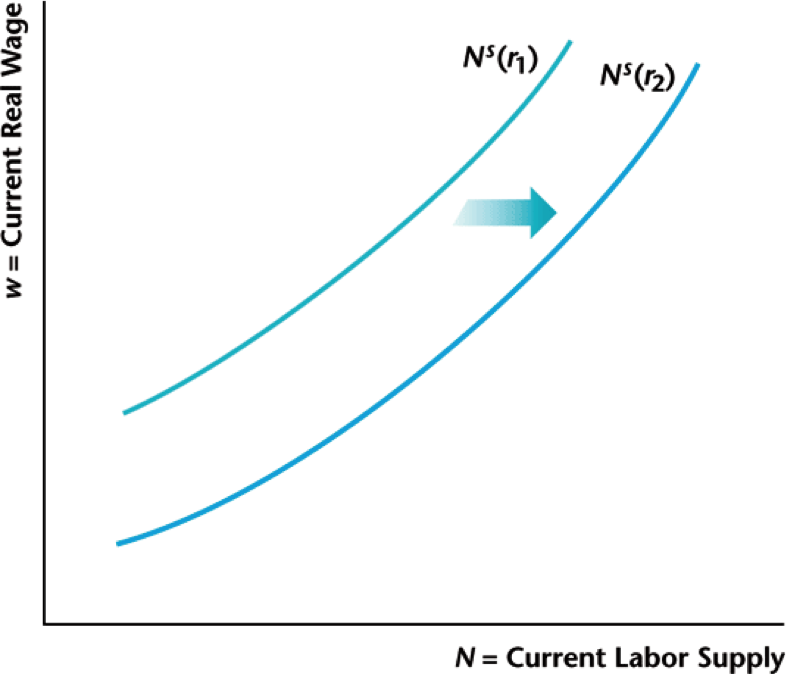
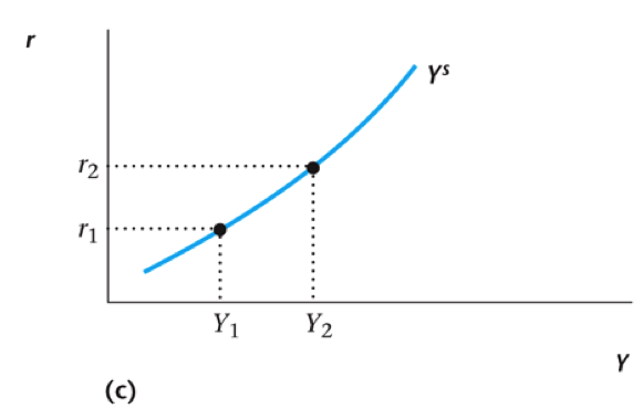
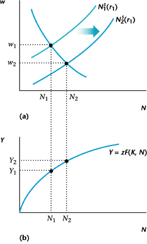
Labor and the Interest Rate

Higher interest rate $\rightarrow$ more labor supplied today

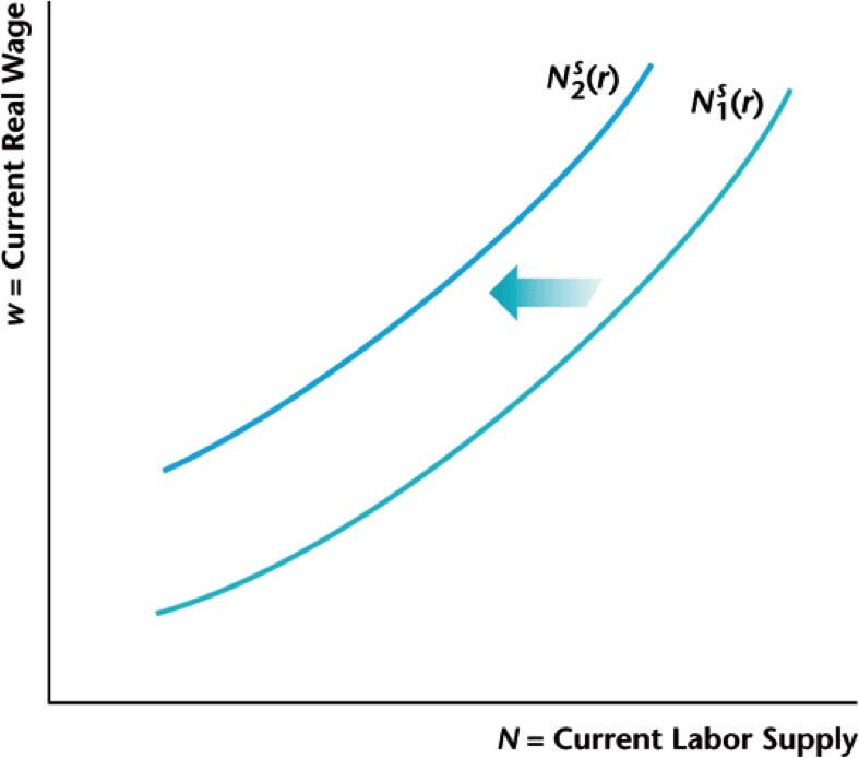
Labor and Wealth

Higher consumer wealth $\rightarrow$ less labor supplied today

Operation of the Firm

• This is much the same as before, except that there are two periods
$$Y = z F(K,N) \qquad \qquad Y^{\prime} = z^{\prime} F(K^{\prime},N^{\prime})$$
• Now the firm is choosing how much to invest in capital ($I$)
$$K^{\prime} = (1-d) K + I$$

Firm Profits and Valuation

• Firms can get $(1-d)K$ from selling off its capital at the end of the second period, so profit in each period is
$$\begin{align*} \pi &= Y - w N - I \\ \pi^{\prime} &= Y^{\prime} - w^{\prime} N^{\prime} + (1-d) K^{\prime} \end{align*}$$
• Combining these two, we can find the present value of the firm (what you might see as a stock price)
$$V = \pi + \frac{\pi^{\prime}}{1+r}$$

Firm Present Value

• Why do firms maximize their present value, instead of something else?
• Firms are owned by consumers, who are free to save/borrow, and hence value securities at present value
• Maximizing "shareholder value" then leads firms to maximize present value
• We could also think about firms themselves borrowing, in which case firms are just maximizing their "wealth"

Firm's Optimal Choices

• Firms will choose investment $I$, as well as employment $N$ and $N^{\prime}$ to maximize value $V$
• We've already seen firm labor before, for that we set
$$MP_{N} = z F_N = w \qquad \qquad MP_{N^{\prime}} = z^{\prime} F_{N^{\prime}} = w^{\prime}$$
• Notice the optimal employment today $N$ depends only on capital today $K$ and the optimal employment tomorrow $N^{\prime}$ depends only on capital tomorrow $K^{\prime}$
• What assumption led to this? In what situations might this not be the case?

Optimal Investment Choice

• The total value of the firm is given by
$$\begin{align*} & V(I,N,N^{\prime}) = zF(K,N) - w N - I \\ & + \frac{z^{\prime}F((1-d)K+I,N^{\prime}) - w^{\prime} N^{\prime} + (1-d) ((1-d)K+I)}{1+r} \end{align*}$$
• So the derivative of $V$ with respect to $I$ is
$$\begin{align*} & \frac{\partial V}{\partial I} = - 1 + \frac{z^{\prime}F_{K^{\prime}} + 1-d}{1+r} = 0 \\ \Rightarrow\ & r = MP_{K^{\prime}} - d \end{align*}$$

Interpreting Interest Rate

• What is the interest rate? It's a price like any other
• It represents the return on investment opportunities
• Consumers lend money to banks $\rightarrow$ banks lend to firms
• Firms buy a machine, operate for a year, sell back: they get more output ($F_{K^{\prime}}$) and the machine is worth a fraction $d$ less next year (resale value)
$$\left[ F(K^{\prime}+\Delta,N^{\prime}) - F(K^{\prime},N^{\prime}) \right] + \left[ (1-d) \Delta - \Delta \right] \\ \downarrow \\ \Delta \left[F_{K^{\prime}} - d\right]$$

Role of Interest Rate

• Since $r$ is a price, it is a signal to actors about what to do
• Consumer's Euler condition: higher interest rate $\rightarrow$ save more! (better return on savings)
• Firms optimality: higher interest rate $\rightarrow$ invest less! (higher borrowing costs)
• In equilibrium, the interest rate equates investment and savings in the aggregate

Brief Note About Graphs

• Supply and demand graphs are the worst
• Whoever decided to put prices on the y-axis was an idiot
• Nonetheless, here we are, and Williamson follows suit
• You can think about this as a supply and demand graph
  • investment decreases with interest rate
  • savings increases with interest rate
  • equilibrium is where they intersect

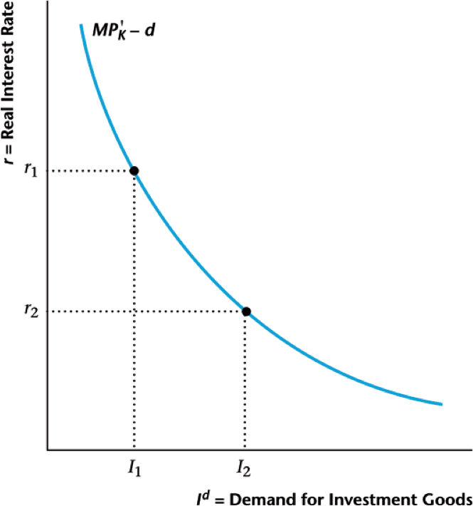
Firm's Investment Behavior

Higher interest rate leads to lower investment

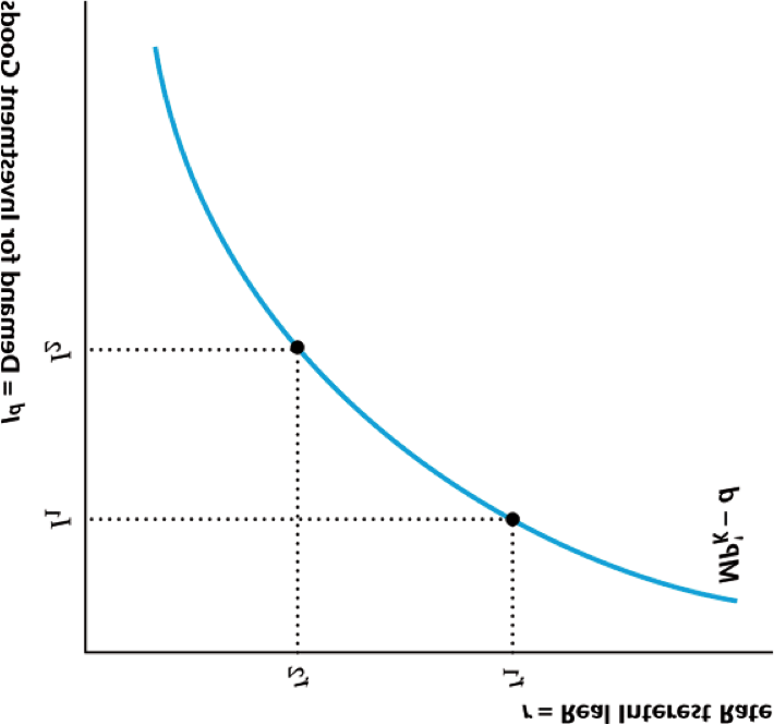
Firm's Investment Behavior

How you should really think about it

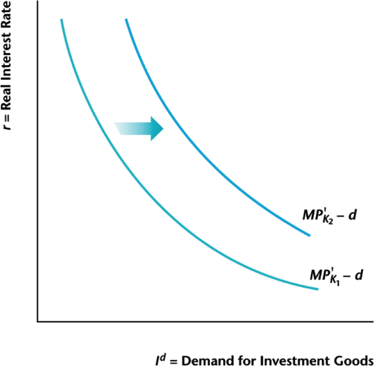
Changes in Investment Behavior

Lower current capital $\rightarrow$ higher investment

Higher future TFP $\rightarrow$ higher investment

Changes in Equilibrium

• What if current capital decreases? Do we just invest proportionally more since
$$r = F_{K^{\prime}}(K^{\prime},N^{\prime}) - d$$
• Lots of moving parts, so it's not that simple!
• To counteract lower $K$, we would increase $I$, but that decreases current consumption
• Decreasing current consumption $c$ breaks Euler equation
$$\frac{c^{\prime}}{c} = 1 + r$$

Labor Market Dynamics

• We've been ignoring labor until now, let's look into it
• Just as the interest rate intermediates savings and investment, the wage ($w$) intermediate the supply and demand for labor
• Consumers: higher wage $\rightarrow$ work more hours, search more
• Employers: higher wage $\rightarrow$ shorten shifts, hire less
• Wage equates supply and demand in each period ($w$ and $w^{\prime}$)

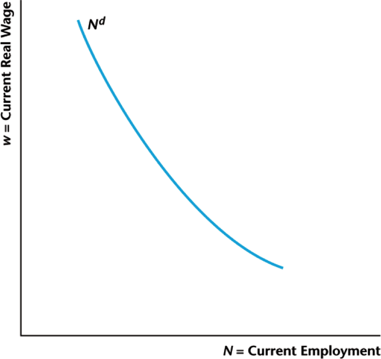
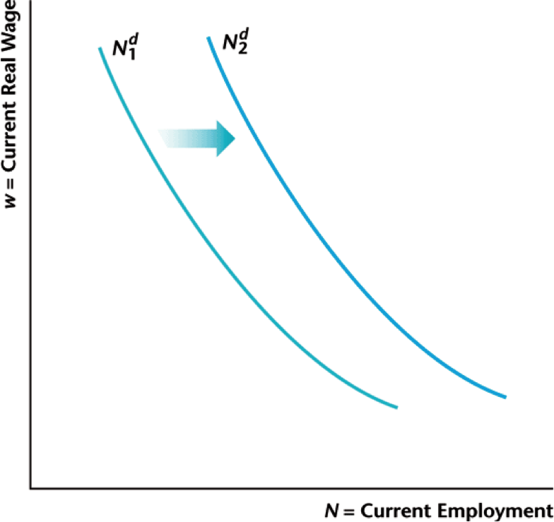
Aggregate Labor Demand

Higher wage $\rightarrow$ less labor demanded

Labor and Capital

• More capital $K$ raises the marginal product of labor
• Think about more machines with the same number of operators
• Clearly increases in total factor productivity $z$ also increase MPL
• If MPL goes up, firms will increase labor demand further until $MPL = w$ again

Labor and Capital

Higher $z$ or $K$ $\rightarrow$ higher labor demanded

Firm Financing Details

• What happens when firms choose large investment?
$$\pi = Y - w N - I \lt 0$$
• Where does firm get money to pay for wages and investment? They borrow
• Recall from consumer side, when there is asymmetric information, borrowing rate might be higher than lending rate
• Same is true for firms: suppose only a fraction of firms $a$ repay loans. Then borrowing rate $r^b$ will be
$$1+r^b = \frac{1+r}{a} \quad \Rightarrow \quad r^b = \frac{1+r}{a} - 1 = F_{K^{\prime}} - d$$

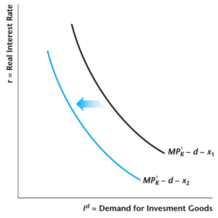
Rising Default Premium

Define default premium $x = r^b - r$

Default premium rises $\rightarrow$ investment demand falls

Time Series Evidence

During recessions: interest rate spreads rise, investment falls

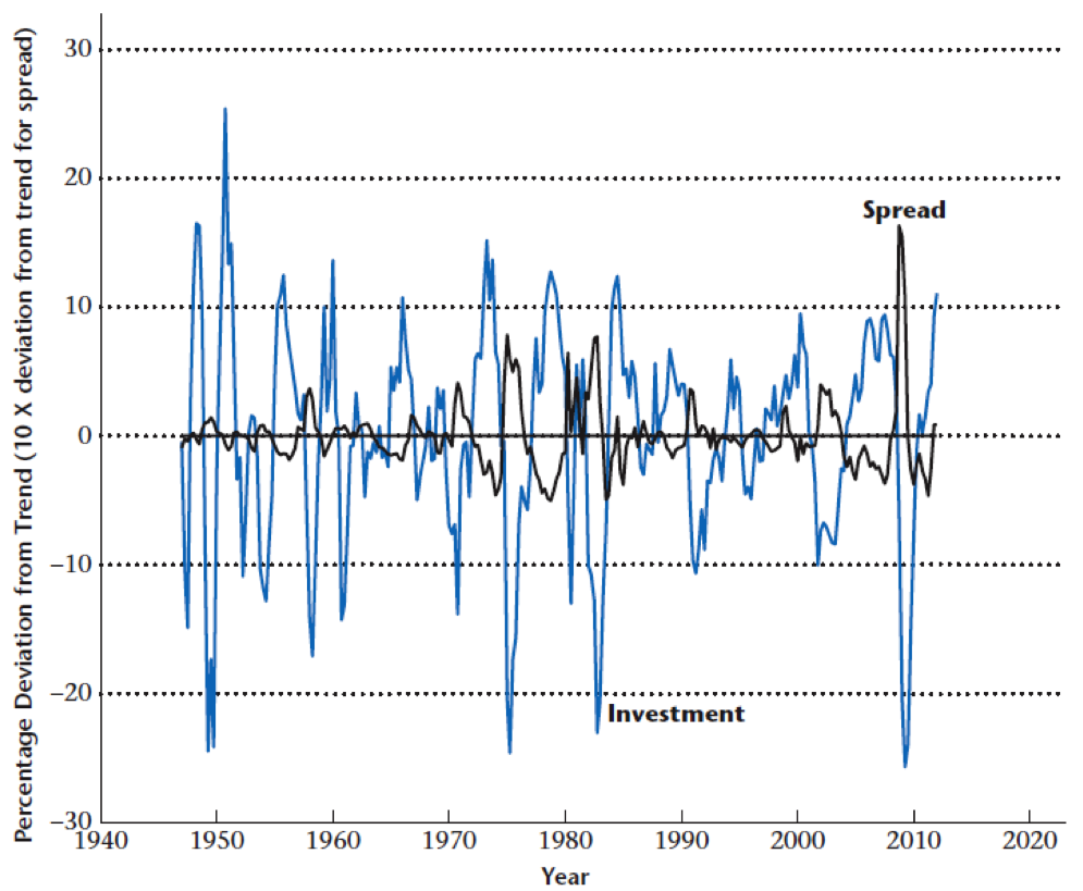
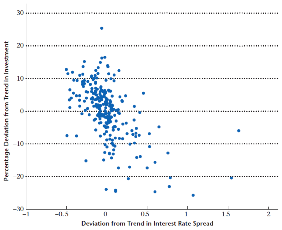
Time Series Evidence

Negative correlation between rate spreads and investment

Role of Government Spending

• As before, government taxes consumers lump sums $T$ and $T^{\prime}$ in each period. No taxes on firms
• Government spending is $G$ and $G^{\prime}$ in each period
• Given that government can borrow and save at rate $r$, lifetime budget constraint is
$$G + \frac{G^{\prime}}{1+r} = T + \frac{T^{\prime}}{1+r}$$

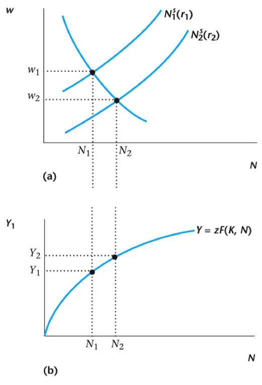
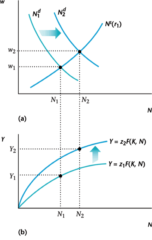
Macroeconomic Equilibrium

• In equilibrium, the interest rate $r$ equates savings and investment and the wages $w$ and $w^{\prime}$ equation labor supply and demand in each period
• Changing even one of these prices affects all three equations, e.g., changing the interest rate changes labor supplied
• We can think about this hierarchically: what if we fix interest rate $r$ and solve labor markets
• This tells us the values of $w$ and $N$ for a given $r$

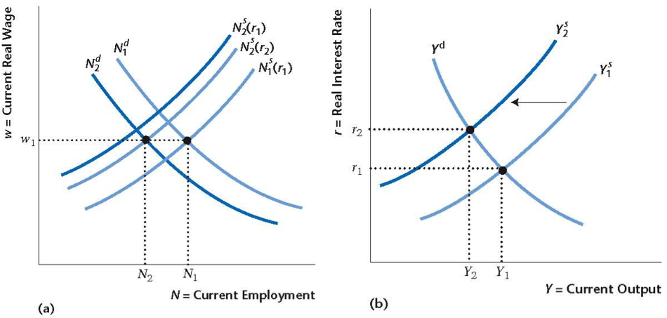
Labor Market Equilibrium

Equilibrium values for wages $w$ and employment $N$

Labor Market Equilibrium

Equilibrium wages and employment for rates $r_1$ and $r_2$

Effect of Government Spending

Gov't spending decreases wealth $\rightarrow$ less leisure, more work

Effect of TFP Increase

Firms demand more labor $\rightarrow$ even higher output

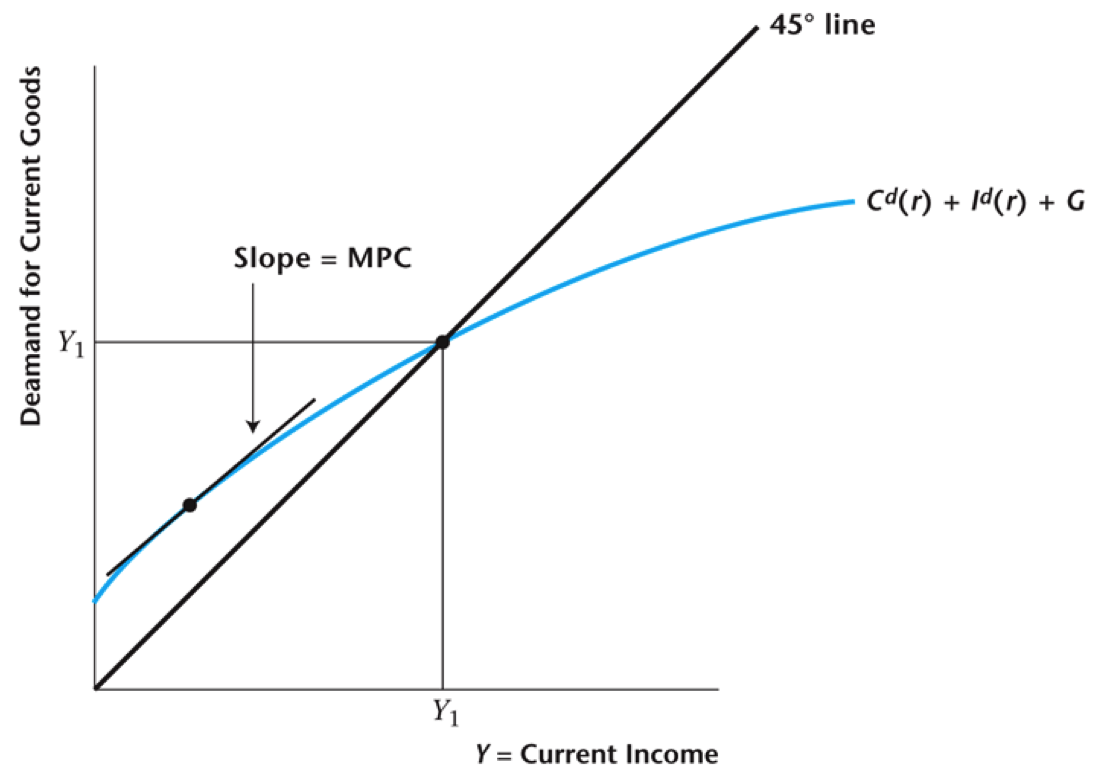
Demand Side for Goods

• Consumer's budget constraint is
$$C + S = w N + \pi - T = Y - I - G$$
• If net savings equals zero ($S = 0$), we get that old GDP saw
$$Y = C + I + G$$
• We can utilize this to define the demand function for current output
$$Y^d(Y,r) = C^d(Y,r) + I^d(r) + G$$

Complications from Wealth

• Supply side of goods market is "easy" because firms don't have wealth effects, only price effects
• Consumers are bit more complicated: we need to keep track of changes in wealth
• What is the wealth of consumers? Depends on output and investment
$$we(Y,r) = Y - I^d(r) - G$$
• Firm decisions give investment $I^d$ for a given interest rate $r$

Accounting for Wealth Effects

$(Y,r) \rightarrow we(Y,r) \rightarrow C^d(Y,r),I^d(r) \rightarrow Y^{\prime}$

Intersection point is where $Y = Y^{\prime}$

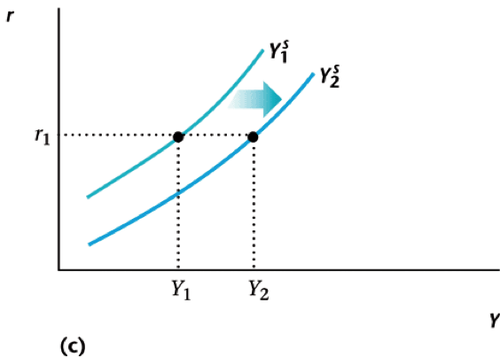
Goods Demand Function

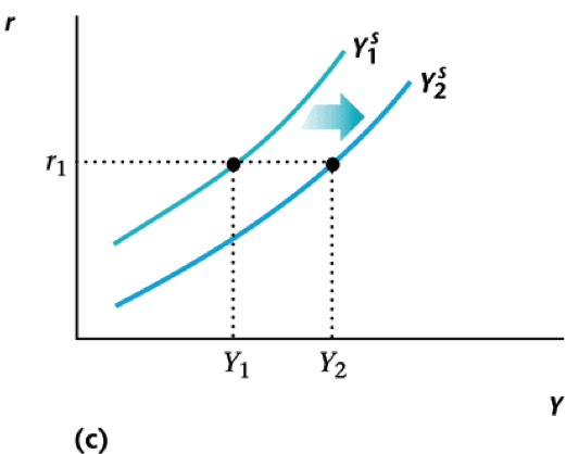
Now we can look at this as a function of $r$

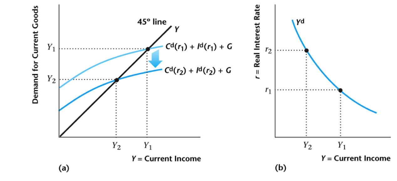
Using Our Intuition

• Outcome is exactly what we would expect from intuition
• For consumers, higher interest rate means more savings, hence less consumption today, so $C^d(r)$ decreasing
• For firms, higher interest rate means less investment, meaning $I^d(r)$ decreasing
• Therefore $Y^d(r)$ also decreasing
$$Y^d(r) = C^d(r) + I^d(r) + G$$

Putting It All Together

Here we have simultaneous goods and labor equilibrium

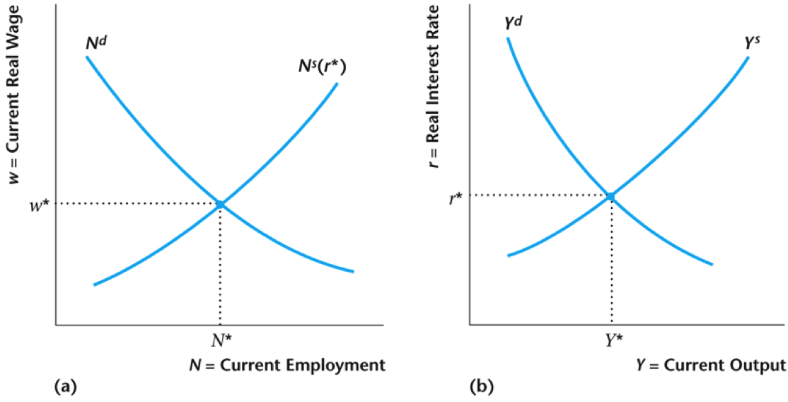
Thinking About Equilibrium

• It makes sense that the wage rate clears the labor market, but what's going on with the interest rate and the supply of goods today?
• You can also think of this as the interest rate clearing the savings/loan market: remember that net savings can be expressed as
$$S(r) = Y^d(r) - C^d(r) - I^d(r) - G$$
• In equilibrium we want to have $S(r) = 0$, since actually the representative has no one to borrow to or from (except maybe the government)

Specific Examples: Investment

• Combining consumer's Euler equation and firm's investment
$$MRS_{C,C^{\prime}} = 1+r = MP_{K^{\prime}} + (1-d)$$
• Let's say that utility is logarithmic and production is Cobb-Douglas
$$u(C,N) = \log(C) + \eta\log(1-N) \\ z F(K,N) = z K^{\alpha} N^{1-\alpha} \\ \Rightarrow \frac{C^{\prime}}{\beta C} = 1 + r = \alpha z^{\prime} \left(\frac{N^{\prime}}{K^{\prime}}\right)^{1-\alpha} + (1-d) \quad ①$$

Specific Examples: Labor

• We can do a similar thing on the labor side, consumer + firm
$$MRS_{N,C} = w = MP_L$$
• Using logarithmic preferences and Cobb-Douglas production
$$\frac{\eta C}{1-N} = w = (1-\alpha) z \left(\frac{K}{N}\right)^{\alpha} \quad ② \\ \frac{\eta C^{\prime}}{1-N^{\prime}} = w^{\prime} = (1-\alpha) z^{\prime} \left(\frac{K^{\prime}}{N^{\prime}}\right)^{\alpha} \quad ③$$

Putting It All Together

• Things like $z$, $K$, and $\alpha$ are all exogenous parameters
• We want to find the endogenous variables, which are
$$I,N,N^{\prime},C,C^{\prime}$$
• We already have three equations for $I$, $N$, and $N^{\prime}$, the last two for $C$ and $C^{\prime}$ are the budget equations
$$C = z K^{\alpha} N^{1-\alpha} - I - G \quad ④\\ C^{\prime} = z^{\prime} (K^{\prime})^{\alpha} (N^{\prime})^{1-\alpha} + (1-d) K^{\prime} - G^{\prime} \quad ⑤$$

Finding a Solution

• So that's fun. We could in principle put these five equations into a computer and find values for the five equilibrium variables
• People (myself included) do this pretty often!
• It's also interesting to look at how the equilibrium variables change when we change the parameters
• To do this we'll rely on graphs: but this is just using intuition to think about these equations

Some Thought Experiments

1. How does a temporary increase in government expenditure affect the economy? ($G$)
2. A decrease in the capital stock (by natural disaster or war) affect the economy? ($K$)
3. A temporary increase in TFP affect the economy? ($z$)
4. What if TFP is expected to increase in the future? ($z^{\prime}$)
5. How do credit frictions affect the economy?
6. What are the effects of sectoral shocks on the economy?

Government Spending Increase

Government Spending Increase

• Primary effect: goods demand $Y^d$ $\uparrow$
• Present value of taxes $\uparrow$ $\rightarrow$ consumers work more $N^s$ $\uparrow$ (income effect)
• More work means less leisure and supply of goods $Y^s$ $\uparrow$
• Can see from graphs that wage $w$ $\downarrow$ and interest rate $r$ could go either way

Spending Multiplier

• The government spending multiplier is that ratio of the change in output to the change in government spending
$$m = \frac{\Delta Y}{\Delta G} = \frac{Y_2 - Y_1}{G_2 - G_1}$$
• Since change in $G$ is temporary, effect on consumer wealth (present value) should be small
• Thus we might think that interest rate $r$ $\uparrow$ and
$$\Delta Y \lt \Delta G \Rightarrow m \lt 1$$

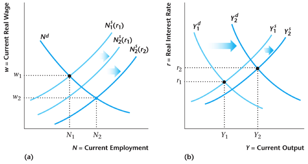
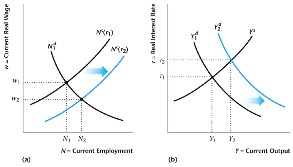
Increase in Current TFP

Increase in Current TFP

• Primary Effect: increase in demand for labor (firms) $\rightarrow$ increase in goods supply
• Second Order: Lower interest rate $\rightarrow$ less labor supply today (lower return on saved wages)
• In the end, output $Y$, wage $w$, and labor $N$ rise. Interest rate $r$ however falls
• This is a boom: in recession, everything happens in reverse

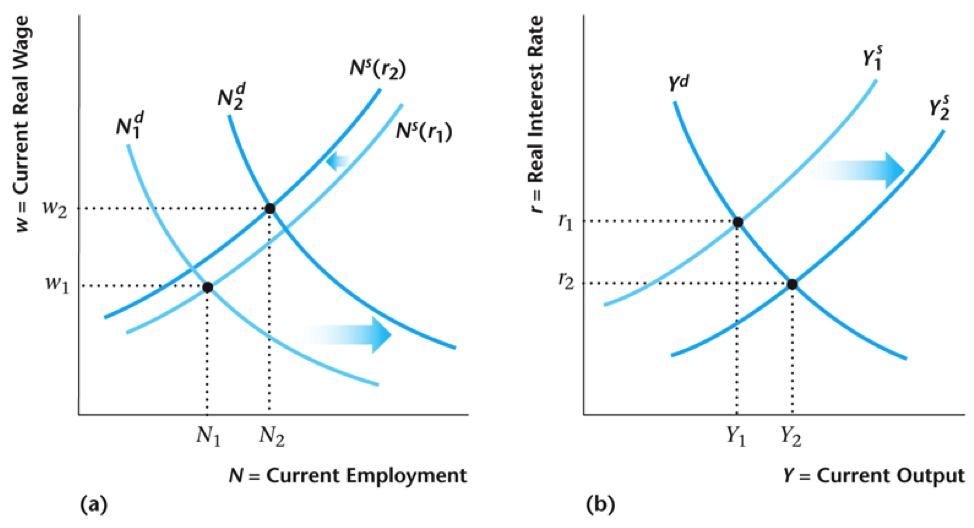
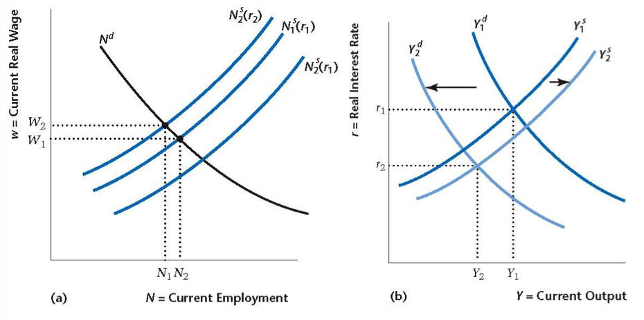
Increase in Future TFP

Changes in Future TFP

• Increase in $MP_{K^{\prime}}$ causes investment $I$ to go up ($Y = C + I + G$)
• This increases interest rate $r$, leading to increase in labor supply $N^s$ today (better savings rate)
• Net effect is higher labor, output, and interest rates, but lower wages today

Expectations About the Future

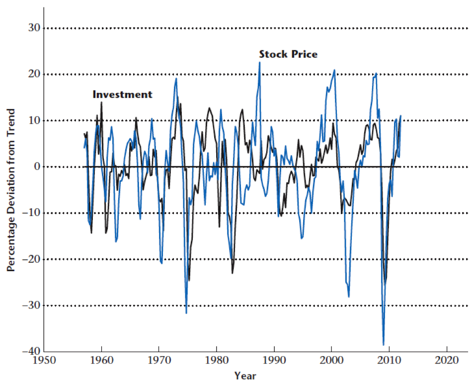
• Financial theory tells us that stock prices act to aggregate information, namely expectations about future profit streams
• Investment and the relative stock price index are positively correlated
• Consistent with the view that fluctuations in news about the future are an important source of business cycles

Data on Stocks and Investment

Stock prices and investment move together

Credit Frictions

• One feature of the recent financial crisis was more severe credit market frictions
• Asymmetric information (higher borrowing rates) and limited commitment (limits on borrowing and collateral)
• In our model, what happens when credit market frictions become more severe?
• Credit constraints will reduce demand for goods, but may also affect how much consumers want to work

Increase in Credit Frictions

Increase in Credit Frictions

• Consumers are more credit constrained so they consume less $Y^d$ $\downarrow$ today
• Lower present value income causes consumers to work more $N^s$ $\uparrow$ which increases supply of goods
• At the same time, lower interest rate $r$ causes consumers to work less $N^s$ $\downarrow$
• Net effect is ambiguous in the end (depends if demand effect is stronger)

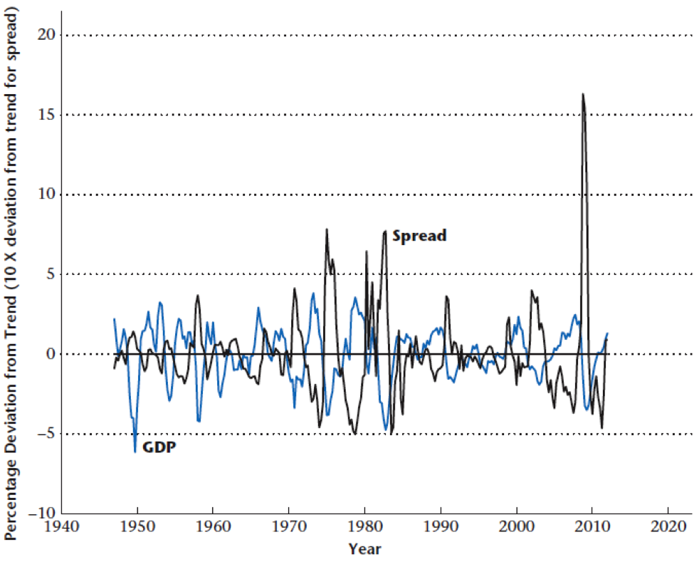
Credit Frictions and GDP

Credit frictions and GDP are negatively correlated

Sectoral Labor Shocks

• “Jobless recoveries” a feature of the last 3 recessions (2008, 2001, and 1991)
• Could be due to sectoral reallocation – changes in labor markets and the structure of production giving rise to movement of labor across sectors
• For example, a negative shock to the manufacturing sector (auto and steel), and a positive shock to the services (health and education)
• Since reallocation takes time, this may show up as a temporary dip followed by growth

Effect of Sectoral Shock

Directly affects labor supply/demand through mismatch

Explanation of Effects

• Sectoral shocks add frictions to the labor market
• More costly for firms to hire, labor demand shifts to the left
• Also more costly for workers to find employment, labor supply shifts to the left
• Output supply shifts to the left, second order effect from increase in interest rate

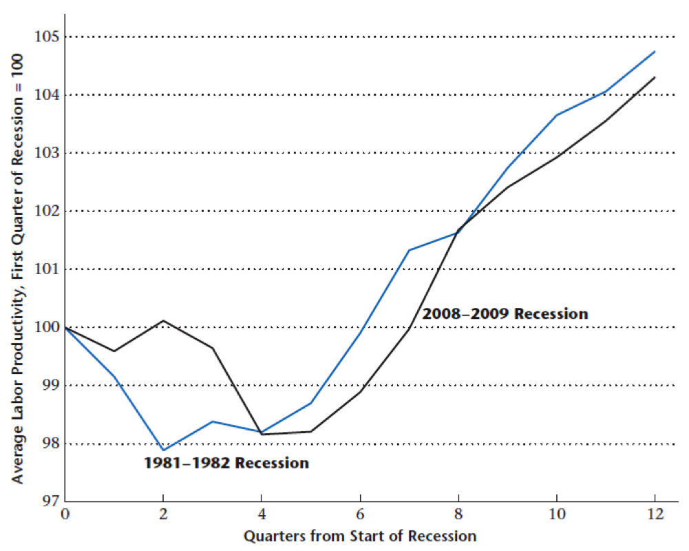
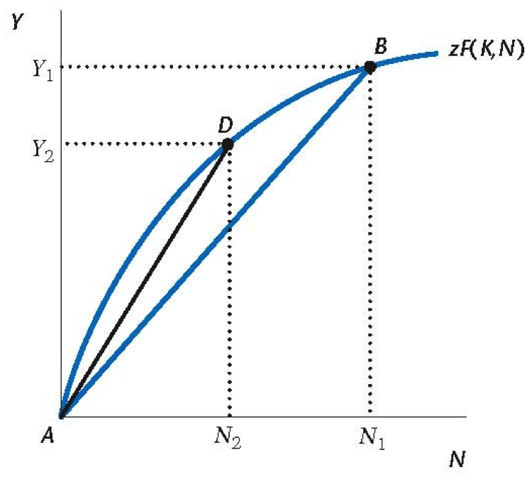
Average Productivity Effect

Employment decreases but output/worker goes up!

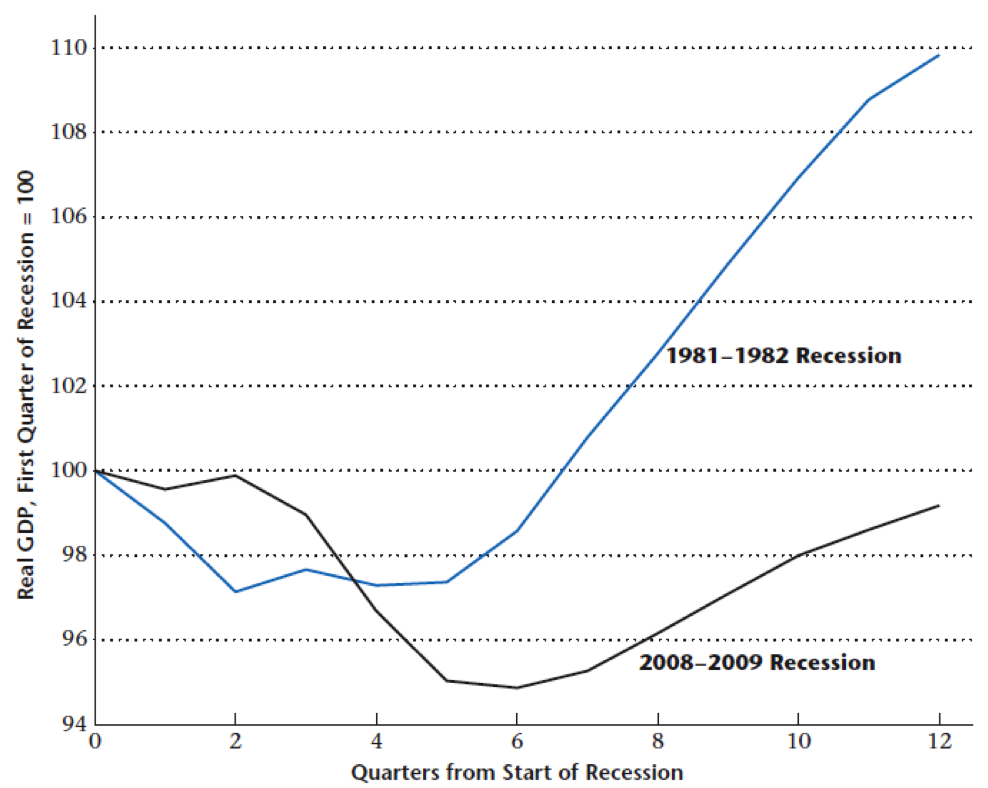
Recent Recession and GDP

Large decline in real GDP

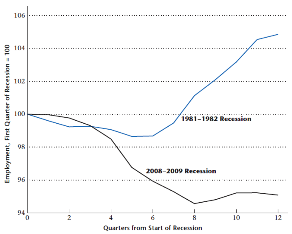
Recessions and Employment

Larger drop in employment and “Jobless Recovery”

Recessions and Productivity

Smaller drop and quick rebound of labor productivity