Intermediate
Macroeconomics

Lecture 4

Economic Growth

In This Lecture

• Why do countries grow economically?
• Why do some countries grow faster than others?
• Why has growth progressed at different rates over time?
• What is the best way to measure growth?

Overview of the Facts

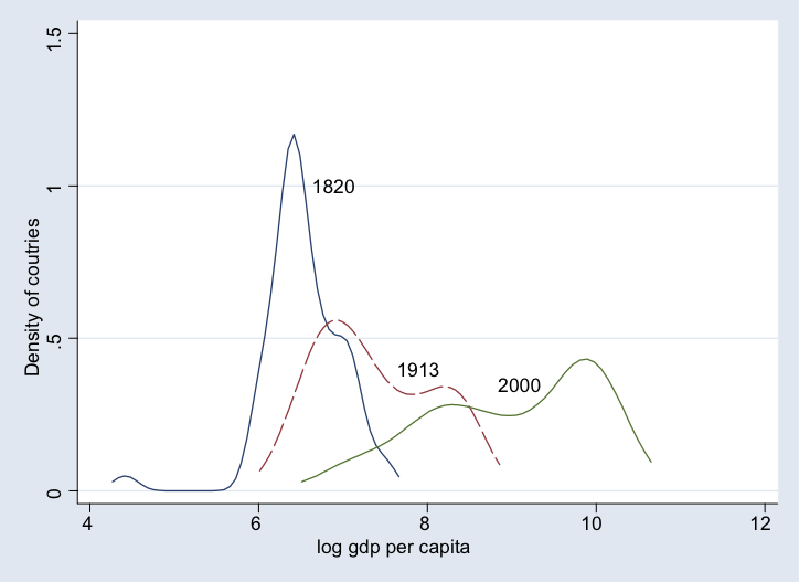
• Growth in living standards was stagnant until about 1800
• During this time, cross-country differences in living standards were small
• Since the industrial revolution, a subset of countries has experienced sustained per capita output growth of about 2%
• Because some countries did not experience this, cross-country differences in per capita output have increased

Growth In The Very Long Run

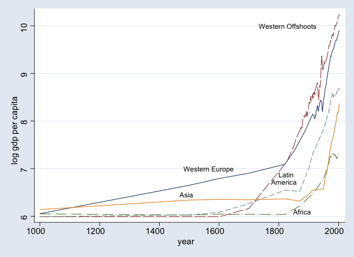
Post Industrial Revolution

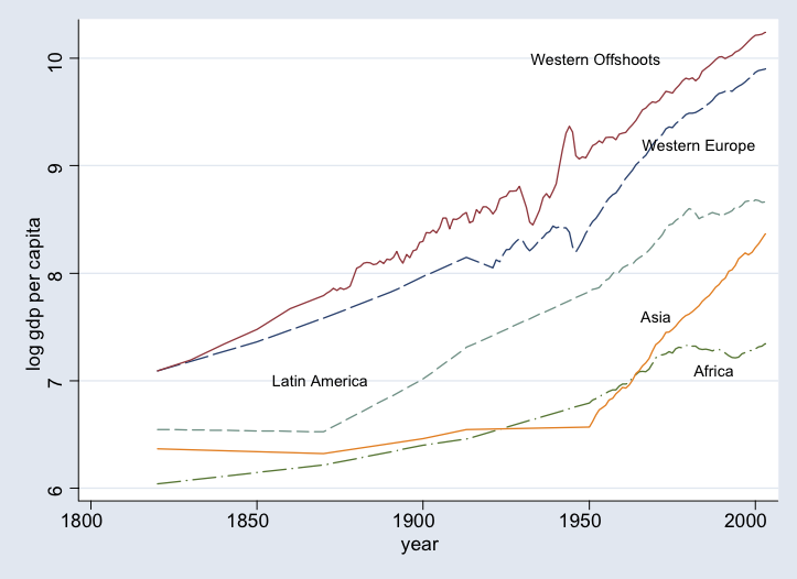
"The Great Divergence"

Two Models of Growth

Malthusian Model

• Plausible and accurate for pre-1800 experience
• Features population growth and fixed supply of land

Solow Model

• Applicable to post-1800 industry led growth
• Features growth in population, technology, and capital

Malthusian Model

Thomas Malthus (1766-1834)

Conceptual Motivation

• We want to make a model of an agrarian society
• Low level of technological advancement
• No substantial capital investment
• No way to control birth or death rates
• Expect a pretty grim outcome

Theoretical Components

• Output is produced from land and labor
$$C = Y = z \cdot F(L,N)$$
• Population growth is a function of birth and death rates
$$N^{\prime} = N(1+b-d)$$
• Assume this varies systematically with per capita income
$$\frac{N^{\prime}}{N} = 1 + b - d = g\left(\frac{C}{N}\right)$$

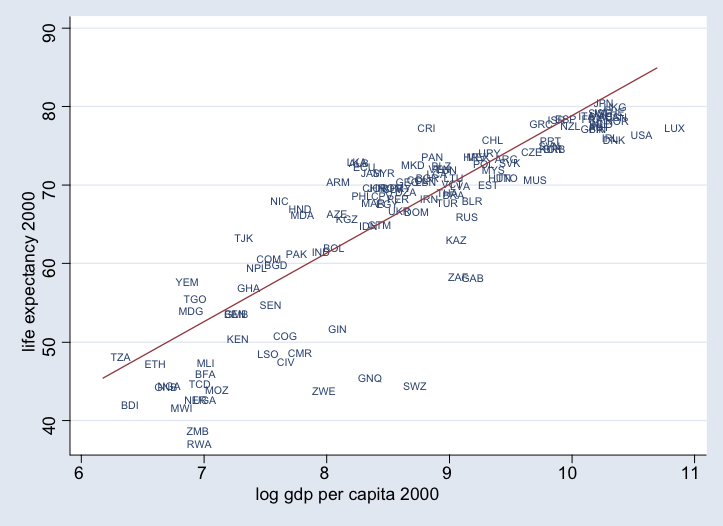
Contemporary Evidence

Life expectancy rises strongly with output per capita

Production Assumptions

• The production satisfies constant returns to scale
$$\frac{C}{N} = \frac{zF(L,N)}{N} = zF(L/N,1)$$
• Define population normalized variables
$$c \equiv \frac{C}{N} \quad \text{and} \quad \ell = \frac{L}{N}$$
• Now we can define $f(\ell) = F(\ell,1)$ so that
$$c = z f(\ell)$$

Steady State Equilibrium

• In equilibrium, we have a constant size population
$$N^{\prime} = N = N^{\ast}$$
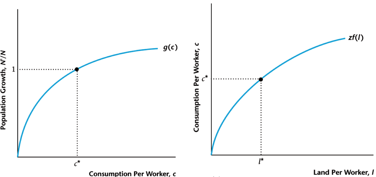
• Using our law for population growth
$$1 = \frac{N^{\prime}}{N} = g\left(\frac{C}{N}\right) = g(c)$$
• This determines a unique value of $c^{\ast}$!

Population Level

• Think about $f(\ell)$ as the production function for a single farm, instead of whole economy $F(L,N)$
• There is no investment, consumption equals output
$$c^{\ast} = z f(\ell^{\ast})$$
• Since land is fixed, this means that
$$\ell^{\ast} = \frac{L}{N^{\ast}} \quad \Rightarrow \quad N^{\ast} = \frac{L}{\ell^{\ast}}$$

Visualizing the Equilibrium

Effect of Tech. Change

• An increase in $z$ pushes up output $C$ and hence output per worker $c=C/N$ rises
• This causes an increase in population growth $N^{\prime}/N=g(c)>1$
• Eventually $N$ grows enough that $c=zf(L/N)$ returns to its original level so that $g(c)=1$
• So new population $N$ is higher and $\ell=L/N$ is lower

Visualizing Tech. Change

Path of Adjustment

No long-term change in consumption (Malthusian trap)

Other Exogenous Changes

• So if technological improvements don't lead to high living standards, what does?
• Population control can do the trick: imagine if the level of the $g$ function shifted downwards
• For any given $c$ we have $g_2(c) \lt g_1(c)$
• This implies $c^{\ast}_2 \gt c^{\ast}_1$ and $\ell^{\ast}_2 \gt \ell^{\ast}_1$, higher living standards
• As a result, lower population $N^{\ast}_2 \lt N^{\ast}_1$

Visualizing Population Control

Escaping the Malthusian Trap

Source: A Farewell to Alms by Gregory Clark

Takeaway From Malthus

• First key element is relationship between income and population growth
• Second key element is fixed supply of land $\rightarrow$ decreasing output per worker
• First one breaks down eventually, but that's fine
• Second can be sidestepped: think buildings and skyscrapers (effective land) or advanced machines (capital)

Working Backwards

• Suppose we knew the exact relationship between income per capita and population growth $g(c)$
• Population growth is much easier to measure historically than output (GDP)
• We could use this to invert $g$ and find output from population growth

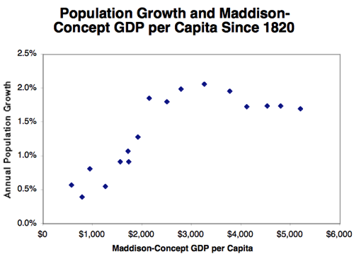
Contemporary Relationship

Looking across countries pre WW II using Maddison data

Implied GDP Series

Using world population estimates from Kremer (1993)

Modern Economic Growth

Moving to Solow's World

• Now we'll take population growth as exogenous
• This is more reasonable at higher income levels (as we just saw)
• Introduce savings/investment and consequent capital accumulation
• First some facts about growth in the modern era

Relative Ranking of Countries

There is almost no change in relative ranking of countries between 1960 and 2000

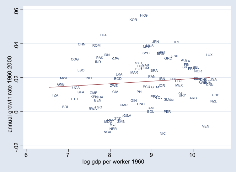
Growth Rates and Output

No relationship between output level and growth rate

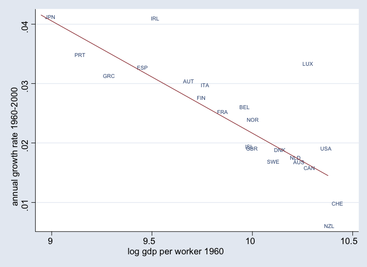
Club Convergence

Restricting to the most advanced countries (core OECD), we see a negative relationship $\rightarrow$ they are converging

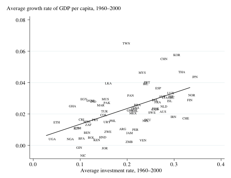
Investment and Output 1

Countries with higher capital investment rates tend to have higher output growth

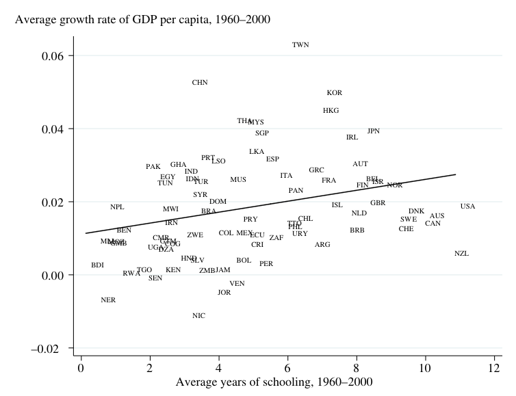
Investment and Output 2

Countries with higher years of schooling tend to have higher output growth

Conceptual Framework

• We make distinction between proximate causes of growth and fundamental causes
• Proximate causes are more tangible and directly observable such as physical and human capital accumulation
• Fundamental causes more amorphous: why did these investment occur? Why don't they occur everywhere?

Solow Model

• Only speaks to proximate causes
• Sustained technological improvement is required for sustained growth in standard of living
• Otherwise, there will be short-term growth, but will eventually plateau

Bulding Blocks: Population

• Population growth is now exogenous at rate $n$
$$N^{\prime} = (1+n) N$$
• This is in line with what we saw before: at some level of income, population growth platueas, then eventually falls

Building Blocks: Savings

• Now we assume that consumers save a constant fraction of their income $s$
$$I = s Y \quad \text{and} \quad C = (1-s) Y$$
• Note that this still satisfies $Y = C + I$
• We ignore the labor/lesiure decision: the consumer works a fixed amount of time (say 8 hours a day)

Building Blocks: Capital

• We're back to useing capital $K$ and labor $N$ as our inputs
• Aggregate production function (representative firm)
$$Y = z F(K,N)$$ $$\Rightarrow \frac{Y}{N} = \frac{z F(K,N)}{N} = z F\left(\frac{K}{N},1\right)$$
• With constant returns to scale, output per worker depends on capital per worker

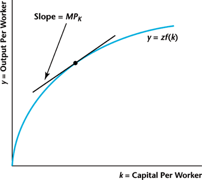
Per Capita Formulation

• Let lowercase variables denote per capita values
$$\frac{Y}{N} = z F\left(\frac{K}{N},1\right) \quad \rightarrow \quad y = z f(k)$$

Investment and Capital

• The capital stock is the total amount of capital in the economy at one time
• It evolves via investment and depreciation
• Making new capital inevitably takes away resources from consumption
• Building steel mill means less steel today for cars (but more steel next year)
• In market setting, these allocations are made through price signals (price of steel)

Evolution of Capital Stock

• We assume that we can take one unit of output and make one unit of capital. This is an assumption!
• Machines break down: capital also depreciates at rate $d$
• Evolution then satisfies
$$\begin{align*} K^{\prime} &= I + (1-d) K \\ &= sY + (1-d) K \\ &= s z F(K,N) + (1-d) K \end{align*}$$

Capital to Labor Ratio

• Rewriting on a per-worker basis
$$\begin{align*} & \frac{K^{\prime}}{N} = s z F\left(\frac{K}{N},1\right) + (1-d)\frac{K}{N} \\ \Rightarrow \quad & \frac{K^{\prime}}{N^{\prime}}\frac{N^{\prime}}{N} = s z F\left(\frac{K}{N},1\right) + (1-d)\frac{K}{N} \\ \Rightarrow \quad & k^{\prime}(1+n) = szf(k) + (1-d)k \\ \Rightarrow \quad & k^{\prime} = \frac{szf(k)}{1+n} + \frac{(1-d)k}{1+n} \end{align*}$$

Steady State Condition

Now that we know how $k$ evolves: look for $k = k^{\prime} = k^{\ast}$

Steady State Properties

• We can see that $k^{\ast}$ is the limiting point starting from any value of $k$
• Rearranging the steady state equation we find
$$szf(k^{\ast}) = (n+d)k^{\ast}$$
• This characterizes the steady state value $k^{\ast}$
• Using this we can see how $k^{\ast}$ changes with the model parameters $s$, $z$, $n$, and $d$

Graphical Characterization

Per worker production equals per worker depreciation

Cobb-Douglas Setting

• What happens if we use the usual production function?
$$Y = z K^{\alpha} L^{1-\alpha} \quad \rightarrow \quad y = z k^\alpha$$
• Steady state $k^{\ast}$ equation
$$\begin{align*} & szk^{\alpha} = (n+d)k \\ \Rightarrow \quad & k^{\ast} = \left(\frac{sz}{n+d}\right)^{\frac{1}{1-\alpha}} \\ \Rightarrow \quad & y^{\ast} = z^{\frac{1}{1-\alpha}} \left(\frac{s}{n+d}\right)^{\frac{\alpha}{1-\alpha}} \end{align*}$$

How Does The Economy Look?

• Both capital per worker $k^{\ast}$ and output per worker $y^{\ast}$ are constant
• Constant standard of living
$$\begin{align*} c^{\ast} &= (1-s) y^{\ast} = (1-s) z f(k^{\ast}) \\ &= (1-s) z^{\frac{1}{1-\alpha}} \left(\frac{s}{n+d}\right)^{\frac{\alpha}{1-\alpha}} \end{align*}$$
• Different from Malthusian outcome: since $Y = N y^{\ast}$, overall economy is growing with population at rate $n$

Changes In Savings Rate

• We take the savings rate $s$ as fixed. Everyone saves a certain fraction of their income (exogenous growth)
• How do things change when we vary the savings rate?
• We can see in the Cobb-Douglas case, steady state capital goes up
$$k^{\ast} = \left(\frac{sz}{n+d}\right)^{\frac{1}{1-\alpha}}$$

Graphical Representation

Investment rises ($s_2 \gt s_1$) $\rightarrow$ higher steady state capital

Algebraic Representation

• We know that the steady state capital level satisfies
$$\begin{align*} & szf(k^{\ast}) = (n+d)k^{\ast} \\ \Rightarrow \quad & s \cdot \underbrace{\frac{zf(k^{\ast})}{k^{\ast}}}_{y/k} = n + d \end{align*}$$
• That ratio is just the average product of capital ($y/k$), which is decreasing when $f$ is concave
• A rise in $s$ means that $k^{\ast}$ must rise to restore equality

Effects of Savings Increase

• Capital per worker $k^{\ast}$ rises, which causes output per worker $y^{\ast}$ to rise
• Investment per worker $i^{\ast} = s y^{\ast}$ will rise, as both terms go up
• But what about consumption per worker? We know $c^{\ast} = (1-s) y^{\ast}$ so ambiguous
• The aggregate growth rate is unchanged: it is still just population growth $n$

Golden Rule Savings Rate

• We know that $s=0$ and $s=1$ lead to $c^{\ast} = 0$, so there should be some savings rate that maximizes $c^{\ast}$
• This is called the golden rule savings rate, we're going to derive it!
• For any $s$, there is some $c^{\ast}(s)$ that results
$$\begin{align*} & c^{\ast}(s) = (1-s)y^{\ast}(s) = (1-s)zf(k^{\ast}(s)) \\ \Rightarrow \quad & \frac{dc^{\ast}}{ds} = (1-s)zf^{\prime}(k^{\ast}) \cdot \frac{dk^{\ast}}{ds} - zf(k^{\ast}) = 0 \end{align*}$$

Golden Rule Derivation

• Okay then, how does $k^{\ast}$ change with $s$? We can use
$$\begin{align*} & szf(k^{\ast}(s)) = (n+d)k^{\ast}(s) \\ \Rightarrow \quad & szf^{\prime}(k^{\ast}) \cdot \frac{dk^{\ast}}{ds} + zf(k^{\ast}) = (n+d) \frac{dk^{\ast}}{ds} \\ \Rightarrow \quad & \frac{dk^{\ast}}{ds} = \frac{zf(k^{\ast})}{(n+d)-szf^{\prime}(k^{\ast})} \gt 0 \end{align*}$$

Golden Rule Derivation

• Putting it all together, we get
$$\begin{align*} & \frac{dc^{\ast}}{ds} = (1-s)zf^{\prime}(k^{\ast}) \cdot \frac{dk^{\ast}}{ds} - zf(k^{\ast}) = 0 \\ \Rightarrow \quad & (1-s)zf^{\prime}(k^{\ast}) \cdot \frac{zf(k^{\ast})}{(n+d)-szf^{\prime}(k^{\ast})} - zf(k^{\ast}) = 0 \\ \Rightarrow \quad & (1-s)zf^{\prime}(k^{\ast}) = (n+d)-szf^{\prime}(k^{\ast}) \\ \Rightarrow \quad & zf^{\prime}(k^{\ast}(s_{GR})) = n + d \\ \end{align*}$$
• Remeber $k^{\ast}$ is increasing in $s$, so there is unique $s_{GR}$

Graphing The Golden Rule

Transition Paths

• Up until now, we've only looked at how things are changing in the steady state, that is in the long-run
• What about in the short and medium term?
• When savings increases, we found that $k^{\ast}$ increased, but growth is the same
• The value of $k$ will change slowly over time from $k_1^{\ast}$ to $k_2^{\ast}$ as capital builds up

Convergence to Steady State

Capital per worker slowly transitions from $k_1^{\ast}$ to $k_2^{\ast}$

Visualizing Transition Paths

• Changes in $K$ come from changes in $k$ and changes in $N$ since $K = k N$
• Population $N$ is always growing at rate $n$ (linear in logs)
$$N_t = N_0 (1+n)^t \quad \rightarrow \quad \log(N_t) = \log(N_0) + t \cdot \log(1+n)$$
• Capital per worker $k$ is on its own transition path
$$k_1^{\ast} = k_0 \rightarrow k_1 \rightarrow k_2 \rightarrow \cdots \rightarrow k_{\infty} = k_2^{\ast}$$

Visualizing Transition Paths

This is what it looks like when you put those two together: $K_t = k_t N_t \quad \rightarrow \quad \log(K_t) = \log(k_t) + \log(N_t)$

What About Consumption?

• The capital level today is always fixed, so it can't jump around too much
• However, when the savings rate changes consumption $c$ can change today
• If savings rate goes up then consumption goes down today
$$c = (1-s) y = (1-s) z f(k)$$
• What about in the long run ($c^{\ast}$)? We saw that depends on whether $s$ is greater or less than the golden rule savings ($s_{GR}$)

Changes in Consumption

Consumption will rebound initially (because $k$ is going up), but long-run depends on savings rate ($s$ vs $s_{GR}$)

Population Growth Changes

What happens when the population growth rate goes up?

Have We Escape Malthus?

• In previous example, population growth rate went up from $2\%$ all the way to $10\%$
• Steady state capital down almost $60\%$, meaning output is down by around $30\%$ (due to decreasing returns)
• That's a pretty Malthusian prediction! What's going on?
• What does this imply about loosening of one-child policy in China?

Technological Change

• Both the savings rate and population growth are inherently bounded
• Savings rate $s \in [0,1]$, and the best we can do for consumption is golden rule rate $s_{GR}$
• Population growth should be at least zero $n>0$, in the long run (otherwise what's the point)
• Neither of these produce sustained growth in livings standards ($c$ or $y$), but technology $z$ is unbounded

Technological Change

Successive improvements in technology $z$ lead to rising $k^{\ast}$

$z_1 = 1 \longrightarrow z_2 = 1.5 \longrightarrow z_3 = 2$

Compare To Malthusian Model

• This is important: for long-term growth in the standard of living, we need continual technological improvement
• In Malthusian world, an increase in technology led to an increase in population growth, so standard of living eventually returned to original value
• Next questions become: how can we measure technology $z$ and what causes it to change over time?

Solow Residual

• Recall earlier when we discussed the Solow residual
• Assuming we know the production function, say
$$Y = z F(K,N) = z K^{\alpha} N^{1-\alpha}$$
• We can use observations of $Y$, $K$, and $N$ to find $z$
$$\hat{z} = \frac{\hat{Y}}{\hat{K}^{\alpha}\hat{N}^{1-\alpha}}$$

Historical Trends in Productivity

Solow Growth Accounting

• One useful exercise is called growth accounting
• Taking logs of the production function, we find
$$\log(Y) = \log(z) + \alpha \log(K) + (1-\alpha) \log(N)$$
• Recall that growth rate = rate of change of log
• So any changes in output $Y$ must come from changes in technology $z$, capital $K$, or labor $N$

Measurement of Capital

• How do we measure capital given so heterogeneous? Use perpetual inventory method
• Assuming depreciation rate (say $d=10\%$), look at how much people are spending on investment
$$K_{t+1} = (1-d) K_t + I_i$$
• Only issues is where do we start $K_0$? We can assume capital starts at a fixed fraction of output
$$\frac{K_0}{Y_0} = \frac{1}{T} \sum_{t=1}^T \frac{K_t}{Y_t}$$

Measurement of Labor

• There are many different ways to measure labor
• Total population, working age population, size of workforce, number of hours worked
• In addition, all of the above but weighted by a measure of human capital (spending, schooling, etc)

Growth In The 20th Century

Looking Across Countries

• We can use to same approach to look across countries, rather than just at the US over time
• This is quite difficult to measure systematically, but the best efforts have been made
• How much of the income differences come from each source?
$$\begin{array}{ll} \textbf{Source} & \textbf{Contribution} \\ \hline \text{Human Capital} & 10-30\% \\ \text{Physical Capital} & 20\% \\ \text{Productivity} & 50-70\% \end{array}$$

Moving Forward

Next task is to figure out where these differences come from