Intermediate
Macroeconomics

Lecture 2

Douglas Hanley, University of Pittsburgh

Theory of Macro

The Walrasian Paradigm

• A Walrasian market is one in which producers and consumers are price takers
• This is reasonable for buying a quart of milk, but probably not so much for, say, buying wind turbines from GE
• Consumers and producers make certain decisions after seeing these prices (supply and demand)
• An equilibrium is a situation where prices are such that the market clears, i.e., supply equals demand

Consumer Optimization Problem

• A consumer has a utility function $u(c_1,c_2)$ which gives a utility value for each $(c_1,c_2)$ combination
• Given market prices $p_1$ and $p_2$, the optimal choice should then be given by
$$\begin{align*} \max_{c_1,c_2} \quad & u(c_1,c_2) \\ \text{subj. to} \quad & p_1 c_1 + p_2 c_2 = p_1 e_1 + p_2 e_2 \end{align*}$$

Lagrangian Techniques

• We want to maximize utility subject to the budget constraint, which says that we must spend less than our wealth
• To do this, we introduce a number ($\lambda$) called the Lagrange multiplier and define the Lagrangian
$$\mathcal{L} = u(c_1,c_2) - \lambda (p_1 c_1 + p_2 c_2 - p_1 e_1 - p_2 e_2)$$
• Think of this as the cost of spending more than you have
• For any given choice of $\lambda \gt 0$, we get values for $(c_1,c_2)$

Finding the Optimum

• To maximize $\mathcal{L}$ for a given $\lambda$ value, we take the derivative with respect to $c_1$ and $c_2$
$$\begin{align*} \frac{\partial\mathcal{L}}{\partial c_1} &= u_1(c_1,c_2) - \lambda p_1 = 0 \\ \frac{\partial\mathcal{L}}{\partial c_2} &= u_2(c_1,c_2) - \lambda p_2 = 0 \end{align*}$$
• Independent of $\lambda$, these two equations imply
$$(\text{MRS}) \quad \frac{u_1(c_1,c_2)}{u_2(c_1,c_2)} = \frac{p_1}{p_2} \quad (\text{Price Ratio})$$

Lagrange Multiplier

• When $\lambda = 0$, we would choose $c_1 = c_2 = \infty$
• When $\lambda = \infty$, we would choose $c_1 = c_2 = 0$
• In-between, there should be some $\lambda^{\ast}$ where the budget constraint is satisfied
$$p_1 c_1(\lambda^{\ast}) + p_2 c_2(\lambda^{\ast}) = p_1 e_1 + p_2 e_2$$
• In practice, we can use budget equation and MRS condition to solve for $c_1$ and $c_2$

Visualizing the Optimum

The MRS is the slope of the indifference curve and the price ratio is the slope of the budget line

Indifference and Substitution

• An indifference curve is a set of points that a consumer is indifferent between
$$u(c_1,c_2) = u(c_1^{\prime},c_2^{\prime}) = \bar{u}$$
• The Marginal Rate of Substitution (MRS) is also the slope of the indifference curve
$$\begin{align*} & \underbrace{u(c_1^{\prime},c_2^{\prime})}_{\bar{u}} \approx \underbrace{u(c_1,c_2)}_{\bar{u}} + \Delta c_1 \cdot u_1 + \Delta c_2 \cdot u_2 \\ \Rightarrow \quad & \frac{\Delta c_2}{\Delta c_1} = -\frac{u_1}{u_2} = -MRS \end{align*}$$

Intuitive Approach

• There is a way to do this without Lagrange by substituting the budget constraint
$$v(c_1) = u\left(c_1,\frac{p_1 e_1 + p_2 e_2 - p_1 c_1}{p_2}\right)$$
• Maximizing this function with respect to $c_2$ yields
$$\frac{\partial v}{\partial c_1} = u_1(c_1,c_2) - u_2(c_1,c_2) \cdot \left(\frac{p_1}{p_2}\right) = 0$$
• Rearranging we find the same MRS condition

Brief Example

• Suppose that the consumer's utility function is
$$u(c_1,c_2) = \log(c_1) + \log(c_2)$$
• The MRS condition is then simply
$$\frac{c_2}{c_1} = \frac{p_1}{p_2} \quad \Leftrightarrow \quad p_1 c_1 = p_2 c_2$$
• Adding in the budget constraint determines our consumption exactly
$$c_1 = \frac{p_1 e_1 + p_2 e_2}{2p_1} \qquad c_2 = \frac{p_1 e_1 + p_2 e_2}{2p_2}$$

An Exchange Economy

• Here we have only two consumers and two goods to keep things simple
• This is an exchange economy: there are no producers, just some goods lying around
• Each consumer $i$ starts with $e^i_1$ of good $1$ and $e^i_2$ of good two
• Consumers can go to the market and buy or sell as much of each good as they wish
• Let $c^i_1$ and $c^i_2$ be what they end up with

Equilibrium Conditions

• Consumers take prices $p_1$ and $p_2$ as given and maximize as we have seen
• There are also market clearing constraints, ensuring all goods are consumed
$$\begin{align*} c^1_1 + c^2_1 = e^1_1 + e^2_1 \quad \text{(Good 1)} \\ c^1_2 + c^2_2 = e^1_2 + e^2_2 \quad \text{(Good 2)} \end{align*}$$

Price Determination

• From the consumer maximization, we know that given $p_1$ and $p_2$, we can find $(c^1_1,c^1_2)$ and $(c^2_1,c^2_2)$
• For random guesses of these prices, it might be that consumers are consuming too much or too little of each good, so our market clearing conditions don't hold
• As with Lagrange multiplier, there should be certain values $p_1^{\ast}$ and $p_2^{\ast}$ such that
$$\begin{align*} c^1_1(p_1^{\ast},p_2^{\ast}) + c^2_1(p_1^{\ast},p_2^{\ast}) = e^1_1 + e^2_1 \\ c^1_2(p_1^{\ast},p_2^{\ast}) + c^2_2(p_1^{\ast},p_2^{\ast}) = e^1_2 + e^2_2 \end{align*}$$

Edgeworth Box

Properties of an Equilibrium

• Because the the MRS of each consumer is equal to the price ratio, they are equal to each other: $MRS_1 = MRS_2$
• It turns out that this is the same condition that ensures Pareto efficiency, thus our equilibrium is efficient
• This result is known as the First Basic Welfare Theorem and can be proven in more general settings as well (many goods and many consumers)

Adding a Macro Flavor

• One of the most important choices that determines macro outcomes is that between consumption and leisure
• Here leisure is defined simply as time not spend working
• Working more means you make more money with which to buy goods, but less leisure time
• There can be interactions: being wealthier can make leisure time more enjoyable
• We model this as a continuous choice, but in reality it is often not continuous or a choice

Theoretical Assumptions

• Now instead of two generic goods, we will have consumption and leisure enter into our utility function $u(c,\ell)$
• Time here is expressed as a fraction between 0 and 1 of the day, month, year, etc.
• Consumers spend a certain fraction of their time $h$ working at wage $w$, so wage income is $w \cdot h$
• The also have capital gains (from firm profits/dividends) $\pi$ and pay taxes $T$ to the government

Consumption-Leisure Choice

• Now the budget constraint for the consumer is
$$c = w h + \pi - T$$
• By assumption, leisure time is that not spent working, so $h = 1 - \ell$, meaning
$$c + w \ell = (\pi-T) + w$$
• This is equivalent to the generic case with $$ \begin{array}{l} p_c = 1 \\ p_{\ell} = w \end{array} \qquad \text{and} \qquad \begin{array}{l} e_c = \pi - T \\ e_{\ell} = 1 \end{array} $$

Optimal Hours Choice

• Avoiding Lagrange multipliers, we can set this up as
$$v(h) = u(wh+\pi-T,1-h)$$
• Taking the derivative we find
$$\begin{align*} & \frac{\partial v}{\partial h} = w u_c(c,\ell) - u_{\ell}(c,\ell) = 0 \\ \Rightarrow \quad & \frac{u_{\ell}(c,\ell)}{u_c(c,\ell)} = w \end{align*}$$
• This is the same MRS condition that we derived before

Graphical Representation

MRS is the slope of the indifference curve.
Wage ($w$) is the slope of the budget set.

How Do Consumers Respond?

• One important question to consider is how consumers respond to changes in: wages ($w$), taxes ($T$), and profits ($\pi$). Sometimes called comparative statics
• Because taxes and profits only affect wealth, they will produce similar and unambiguous responses
• We will generally assume that both consumption and leisure are normal goods, meaning you consume more of them when your wealth increases

Changes in Wealth

Both consumption and leisure rise when $T$ falls or $\pi$ rises

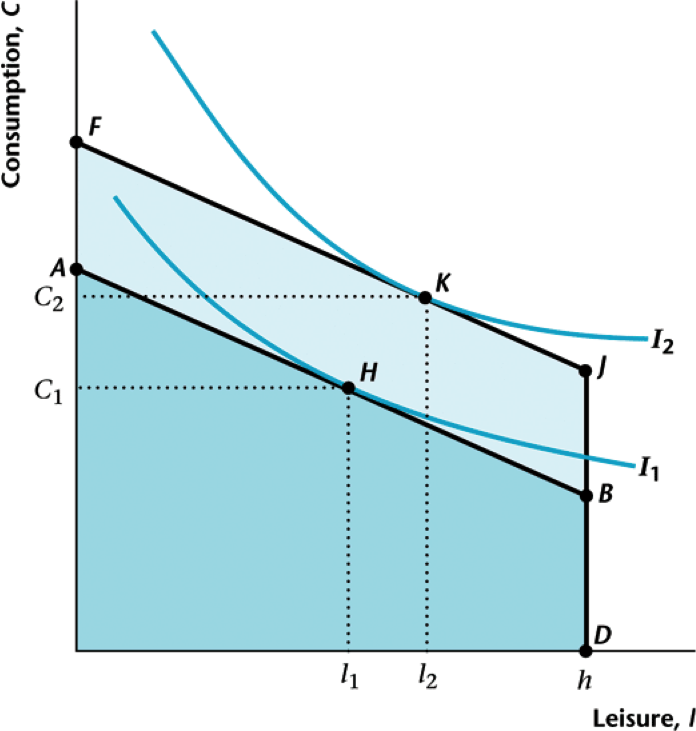
Changes in Wage

Here we see both a wealth effect ($F \rightarrow O$) and a substitution effect ($O \rightarrow H$) when wage rises

A Specific Example

• Let the utility function of the consumer be of the Cobb-Douglas form
$$u(c,\ell) = \log(c) + \eta \log(\ell)$$
• The parameter $\eta$ measures how much this person values leisure, called Frisch elasticity
• Satisfies Inada condition: marginal utility at $c=0$ or $\ell=0$ is infinity $\rightarrow$ will always consume at least a small amount
• Same budget constraint as before
$$c = wh + \pi - T$$

Finding the Optimum

• Simplifies to a choice of hours
$$v(h) = \log(wh+\pi-T) + \eta \log(1-h)$$
• Taking the derivative yields
$$\begin{align*} & 0 = \frac{w}{wh+\pi-T} - \frac{\eta}{1-h} \ \Rightarrow \ h = \frac{1}{1+\eta} - \frac{\eta}{1+\eta}\left(\frac{\pi-T}{w}\right) \end{align*}$$
• Now we can solve for the consumption and leisure too
$$ c = \left(\frac{1}{1+\eta}\right) (w+\pi-T) \quad \ell = \left(\frac{\eta}{1+\eta}\right) \frac{w+\pi-T}{w} $$

Important Implications

• If $w \le \eta(\pi-T)$, the worker chooses $h=0$
• In this setting, hours worked increases with the wage (and leisure consequently decreases)
• As predicted, both consumption and leisure increase with base income ($\pi-T$)
• When base income is zero, hours worked is constant, $1/(1+\eta)$, and invariant to wage!
• When might we expect hours to be decreasing with wage?

Alternative Tax Regimes

• Most taxes we see in the wild are proportional rather than lump-sum
• Consider a consumption (sales) tax $\tau_c$ and a labor (income) tax $\tau_h$
$$c = wh + \pi - \tau_c c - \tau_h wh$$
• Now our utility of working $h$ is expressed as
$$v(h) = u\left(\frac{(1-\tau_w) wh + \pi}{1+\tau_c},1-h\right)$$

Proportional Tax Optimum

• The optimal choice will then satisfy
$$\frac{d v}{dh} = u_c(c,\ell) \left(\frac{1-\tau_w}{1+\tau_c}\right) w - u_{\ell}(c,\ell) = 0$$
• Rearranging we find
$$MRS = \frac{u_{\ell}(c,\ell)}{u_c(c,\ell)} = \left(\frac{1-\tau_w}{1+\tau_c}\right) w$$
• The proportional taxes act the same as changing the wage directly (income and substitution effect)

Back to Cobb-Douglas

• Returning to our specific example, we find
$$v(h) = \log\left[\frac{(1-\tau_w)wh + \pi}{1+\tau_c}\right] + \eta\log(1-h)$$
• Consumption tax $\tau_c$ has no effect! Just scales down consumption. Wage tax $\tau_w$ same as wage $w$
$$h = \frac{1}{1+\eta} - \frac{\eta}{1+\eta} \left[\frac{\pi}{(1-\tau_w)w}\right]$$

Mapping to the Aggregate

• Final conceptual leap is to proclaim this the representative consumer
• Imagine an economy populated with identical replicas of this person
• Aggregate outcomes the same as individual choices
• Each agent is so small, he or she exerts no market power $\rightarrow$ Walrasian assumptions hold

The Production Side

• Consumers are on the demand side for consumption and the supply side for labor
• Now we introduce producers to serve the opposing roles: supply side for consumption and demand side for labor
• Producers have no utility, we assume for now that they act to maximize profits (an approximation of US law, fiduciary duty)

Architecture of a Firm

• Firms take capital $k$ and labor $h$ as inputs and output a consumption good $y$
• Think of a firm as being characterized by a production function
$$y = z \cdot f(k,h)$$
• The term $z$ is called total factor productivity and denotes the total level of output capacity

What is capital?

• Any persistent (durable) machine that is used in the course of production
• Harvester on a farm, tools in a factory, computers in services
• Closely linked with investment because we must forgo consumption to make capital
• There is also intangible capital like inventions, designs, brands, trademarks, etc, which operates similarly

Properties of Production Functions

• Returns to scale: how does doubling all inputs (capital and labor) affect output?
• Decreasing returns: $f(x\cdot k,x\cdot h) \lt x \cdot f(k,h)$
• Constant returns: $f(x\cdot k,x\cdot h) = x \cdot f(k,h)$
• Increasing returns: $f(x\cdot k,x\cdot h) \gt x \cdot f(k,h)$
• All are potentially interesting, though we will generally focus on constant returns

Constant Returns to Scale

• Important to consider the level of aggregation, returns to scale are not necessarily invariant
• Suppose we can build an auto plant for $\$10$ million and each car costs $\$10,000$ to make
• Building 100 cars costs $\$11$ million, while building 200 cars costs $\$12$ million $\lt$ $\$22$ million (increasing returns)
• However, simply building two plants and doubling the number of cars produced is constant returns

Non-constant Returns to Scale

• Increasing and decreasing returns to scale generally involve some sort of externality
• Increasing: at the city level, it is plausible to believe that being in a larger city can enhance the productivity of certain types of workers $\rightarrow$ agglomeration
• Decreasing: conversely, there is also the possibility of clogged roads, noise, or litter $\rightarrow$ congestion
• At the national or global level, the presence of a shared knowledge pool can induce increasing returns

Profit Maximization Problem

• Given a certain amount of capital $k$, a firm hires workers $h$ at wage $w$
• You can think about $h$ as a total number of workers or hours
• With output price $1$, the total profit of a firm is then
$$\pi(h) = z f(k,h) - w h$$
• Taking the derivative, the optimality condition is then
$$MPL = z f_{h}(k,h) = w$$

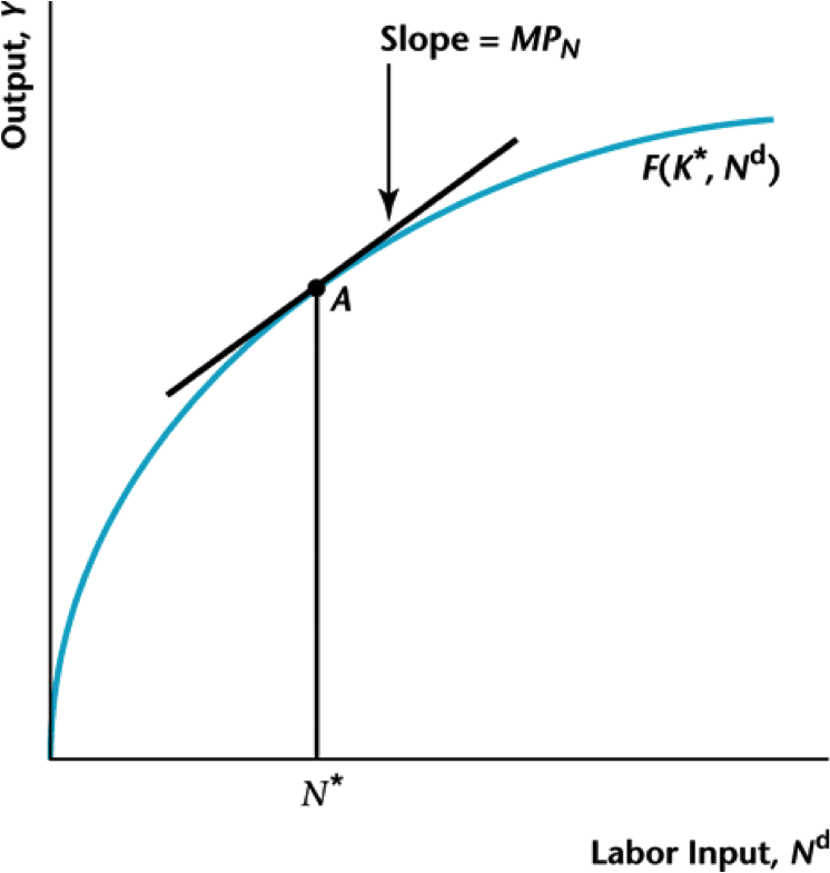
Visualizing the Optimum

The firm hires workers until the marginal product of an additional work is equal to the wage

Properties of the Optimum

• For this to work, we need to have $f_{hh} \lt 0$, decreasing returns, at least eventually
• How does optimal choice $h^{\ast}$ change with $z$, $k$, $w$?
• Given $z f_{h}(k,h^{\ast}(k)) = w$, we can derive
$$ z\left[f_{kh} + f_{hh} \frac{dh^{\ast}}{dk}\right] = 0 \quad\Rightarrow\quad \frac{dh^{\ast}}{dk} = - \frac{f_{kh}}{f_{hh}} \gt 0 $$
• We generally assume that more capital raises the marginal product of labor (MPL), i.e., $f_{kh} \gt 0$

Fixed Costs of Production

• With fixed cost $C$, profit is then
$$\pi = z f(k,h) - w h - C$$
• Calculus is the same as before, but we need to check whether production is "worth it"
• Let $h^{\ast}$ be the optimal choice satisfying $z f(k,h^{\ast}) = w$
• Do we have
$$z f(k,h^{\ast}) - w h^{\ast} > C \quad \text{?}$$

Specific Production Example

• Once again we will use a Cobb-Douglas function
$$y = z k^{\alpha} h^{1-\alpha}$$
• You can verify that this satisfies $f_{kk} \lt 0$, $f_{hh} \lt 0$, and $f_{kh} \gt 0$. The marginal product of labor is then
$$z f_{h} = (1-\alpha) z k^\alpha h^{-\alpha} = (1-\alpha) z \left(\frac{k}{h}\right)^{\alpha}$$

Properties of Optimal Labor

• Using $zf_{h} = w$, we then find the optimal choice of labor
$$h^{\ast} = \left[\frac{(1-\alpha)z}{w}\right]^{1/\alpha} k$$
• Notice that the optimal choice involves targeting a certain ratio of labor to capital. If we all the sudden got more capital, we would hire proportionately more workers
• Total output is computed to be
$$y^{\ast} = z^{1/\alpha}\left[\frac{1-\alpha}{w}\right]^{\frac{1-\alpha}{\alpha}} k$$

Labor Share of Income

• Notice that with Cobb-Douglas, the ratio of labor income to output is
$$\frac{wh}{y} = \frac{f_{h}h}{y} = 1-\alpha$$
• Looking at this in the data we find that in the US, it is quite stable at around $70\%$, meaning $\alpha = 30\%$
• This was actually the impetus for Paul Douglas proposing this functional form
• In some developing countries and more recently in US, labor share has been decreasing slightly

Labor Share Over Time

The labor share in the US has been roughly constant over time

Labor Share Internationally

Internationally labor share has decreased, some substantially

Solow Residual

• This measure is named after Robert Solow, and is given by
$$\hat{z} = \frac{y}{k^{\alpha}h^{1-\alpha}}$$
• The underlying idea is that real GDP combines productivity and investments in capital and labor, while this looks only at the former
• We'll look at better ways to measure this and theories regarding its evolution later in the course

Growth in TFP

Can use observations of $y$, $k$, and $h$ to estimate TFP ($z$)

International TPF Levels

Can see whether growth from TFP or factor accumulation

Capital Investment

Investment also an important driver of output

Moving Forward

• The next step is to declare this firm the representative firm and fuse the consumer and producer work we've done into a full-blown economy
• With this, we can start discussing the determination of wages/prices and allocations
• We can also talk about efficiency and the effects of policy
• Ultimately, we'll want to include capital investment choices and TFP growth

Aggregate Accounting

• We will assume that the government has a balanced budget so that $G=T$
• Combining the consumption and production side, our GDP identities hold
$$\begin{align*} & c = w h + \pi - T = wh + \pi - G \\ & \pi = z f(k,h) - w h = y - w h \\ \Rightarrow \quad & y = c + G \end{align*}$$
• Here we have $I = 0$ and $NX = 0$

Equilibrium Conditions

• Combining optimality conditions, we find
$$\begin{align*} \text{MRS} = &w = \text{MPL} \\ \frac{u_{\ell}(c,\ell)}{u_c(c,\ell)} = &w = z f_h(k,h) \end{align*}$$
• Combined with $c + G = z f(k,h)$ and $\ell + h = 1$, we can fully determine the equilibrium

Cobb-Douglas Example

• Recalling our previous derivations, we have
$$\begin{align*} & \text{MRS} = \frac{\eta c}{\ell} = w = \frac{(1-\alpha) y}{h} = \text{MPL} \\ \Rightarrow \quad & \frac{\eta(y(h)-G)}{1-h} = \frac{(1-\alpha)y(h)}{h} \end{align*}$$
• This is difficult to solve, but when $G = 0$ we get
$$h = \frac{1-\alpha}{\eta + 1-\alpha}$$

Visualizing the Equilibrium

$\eta=1$, $\alpha=0.3$, $G=0.1$

Is This Efficient?

• To determine if this outcome is efficient, consider a social planner who decides the outcome
• Planner chooses $h$, which determines $y$, $c$, $\ell$, and hence utility
• Objective is to maximize agents utility. Could also think of this as agent owning the factory
$$u(h) = u(z f(k,h) - G,1-h)$$
• We still take government spending as given, necessary basic spending

Social Planner's Optimum

• Taking the derivative, we find
$$\begin{align*} & u_c(c,\ell) \cdot z f_h(k,h) - u_{\ell}(c,\ell) = 0 \\ \Rightarrow \quad & \frac{u_c(c,\ell)}{u_{\ell}(c,\ell)} = z f_h(k,h) \end{align*}$$
• The same condition we saw in the equilibrium! So this is the efficient outcome
• Notice that we haven't made any statements about the efficient level of $G$

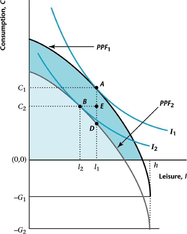
Effect of Changing G

Pure income effect $\rightarrow$ both $c$ and $\ell$ fall

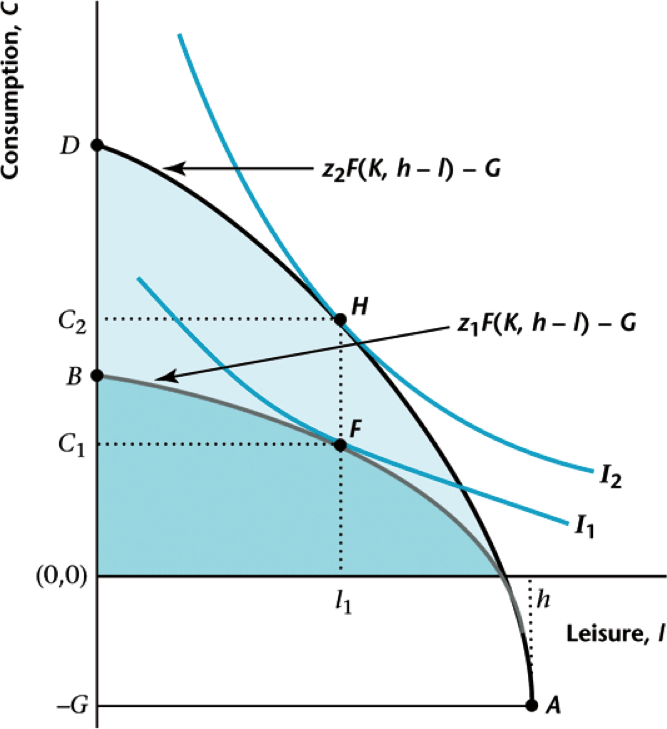
Effect of Changing z

Both income and substitution $\rightarrow$ change in $\ell$ ambiguous

Interpretation of Results

• Change in $G$ is same story as change in $T$ on consumer side
• Change in TFP ($z$) similar to change in $w$ on consumer side
• These forces are candidates drivers for short-term economic fluctuations
• The question is whether they can be treated as exogenous factors and how well they correlate with changes in GDP
• If they do correlate, does that imply causality?

TFP as Driver?

Trouble is that TFP is measured from GDP