Lecture 1: Neoclassical Growth

Solow Growth Accounting

The Solow model is a mathematical embodiment of the above decomposition. It assumes a single aggregate production function describing how inputs capital ($K$), labor ($L$), and technology ($A$) are combined to produce final good $Y$ according to Y = F(A,K,L) Even before we go into specifying agents and their incentives, this allows us to decompose changes in output into changes coming from each of the three inputs. Taking the total derivative, we find \dot{Y} = \dot{A} \frac{\partial F}{\partial A} + \dot{K} \frac{\partial F}{\partial K} + \dot{L} \frac{\partial F}{\partial L} where ``dot'' denotes the time derivative. We can get a bit more traction if we assume a functional form for production. Using a Cobb-Douglas production function given by F(A,K,L) = AK^{\alpha}L^{1-\alpha} we then arrive at a true growth rate decomposition \frac{\dot{Y}}{Y} = \frac{\dot{A}}{A} + \alpha \left(\frac{\dot{K}}{K}\right) + (1-\alpha) \left(\frac{\dot{L}}{L}\right) Alternatively, we can go with a more general constant elasticity of substitution (CES) production function given by F(A,K,L) = A \left[\alpha K^{\frac{\sigma-1}{\sigma}} + (1-\alpha) L^{\frac{\sigma-1}{\sigma}}\right]^{\frac{\sigma}{\sigma-1}} This nests multiple familiar functional forms \sigma \rightarrow 0 \quad \align \Rightarrow \quad \text{Leontieff} \\ \sigma \rightarrow 1 \quad \align \Rightarrow \quad \text{Cobb-Douglas} \\ \sigma \rightarrow \infty \quad \align \Rightarrow \quad \text{Linear} Performing the same decomposition as before, we find \frac{\dot{Y}}{Y} = \frac{\dot{A}}{A} + \bar{\alpha} \left(\frac{\dot{K}}{K}\right) + (1-\bar{\alpha}) \left(\frac{\dot{L}}{L}\right) where \bar{\alpha} = \frac{\alpha K^{\frac{\sigma-1}{\sigma}}}{\alpha K^{\frac{\sigma-1}{\sigma}}+(1-\alpha)L^{\frac{\sigma-1}{\sigma}}} Thus the growth contribution from each factor will be determined jointly by the exogenous factor loadings and the potentially endogenous relative abundance of each factor.

Often it will be useful to express this relationship in per capita terms. We say that a particular production does not feature scale effects if we can express y = f(A,k) where lower case letters are used to denote per capita figures (note that $A$, being non-excludable, has no meaningful per capita analogue). In the general CES setting, this leads us to y = A \left[\alpha k^{\frac{\sigma-1}{\sigma}}+(1-\alpha)\right]^{\frac{\sigma}{\sigma-1}}

Consumers

One of the major simplifying assumptions we'll be making, at least initially, is that of a representative agent. Naturally, with homogeneous agents, this is not a major assumption. When we start introducing heterogeneity amongst agents, for instance between skilled and unskilled labor, this will be more of an issue since different agents can have different responses that do not aggregate linearly. Sometimes you'll see papers that have a single representative household with heterogeneity amongst the agents in the household.

Let's say this agent has the instantaneous utility function $u(c)$ which is then aggregated over time with discount rate $\rho$ U(\mathbf{c}) = \int_0^{\infty} u(c(t)) \exp(-\rho t) dt The consumer have access to a risk-free bond garnering interest rate $r$. Denote their holdings of this asset, which depreciates at rate $\delta$, be denoted by $a$ and the investment rate be $i$. They also have one unit of labor that they supply inelastically yielding wage $w$. The budget equation is then c + i = ra + w In general, we would also include income from firm profits ($\pi$), but because we assume constant returns to scale in production, firms will make zero profits anyway. We can now write down the optimization problem for the consumer. This constitutes the choice of a consumption path $\mathbf{c}$ and investment path $\mathbf{i}$ that maximizes $U(\mathbf{c})$.

This infinite dimensional optimization is not a trivial one. I'm going to skip directly to the recursive formulation. I'll also take this opportunity to provide a little primer on working in continuous time, as opposed to discrete time. Let the current time be $t$ and the next "instant" in time be $t+\Delta$, where $\Delta$ is presumed to be small. Let the present value of having asset level $a$ at time $t$ be given by $V(a,t)$, then we have V(a,t) = \align \max_{c,i} \left\{\Delta u(c) + \exp(-\Delta\rho) V(a+\Delta(i-\delta a),t+\Delta)\right\} \\ \align \quad \text{subj. to } c + i = ra + w Subtracting $\exp(-\Delta\rho)V(a,t)/\Delta$ from both sides, we find \left[\frac{1-\exp(-\Delta\rho)}{\Delta}\right] V(a,t) = u(c) + \exp(-\Delta\rho) \left[\frac{V(a+\Delta(i-\delta a),t+\Delta)-V(a,t)}{\Delta}\right] Taking the limit as $\Delta \rightarrow 0$ yields \rho V = u(c) + (i-\delta a)V_a + \dot{V} where subscripts denote non-time derivatives. In this case the $\dot{V}$ will be zero, as there is no explicit time dependence. The agent's state can be fully described by $a$. So finally we have \rho V = u(c) + (i-\delta a)V_a

Producers

The final good is produced by a continuum of competitive firms. Because we will assume constant returns to scale, it is just as well to consider the case of a single firm that takes prices as given. We will ignore growth in $A$ for now. Because the population is fixed at $1$, aggregate and per capita variables will coincide, so we can just use lower case letters. As before, let the production function be $y = f(k,\ell)$.

The producer faces the following static optimization problem in which they rent capital from consumers and hire them as laborers in order to produce \max_{k,\ell} \left\{f(k,\ell) - rk - w\ell\right\} This yields these simple first order conditions f_k = r \qquad \text{and} \qquad f_{\ell} = w

Optimization

We can derive an analogous expression for the first-order condition in discrete time \Delta u_c(c) = \exp(-\Delta\rho) \Delta V(a+\Delta(i-\delta a),t+\Delta) Canceling terms and taking the limit as $\Delta \rightarrow 0$ yields simply u_c = V_a Not coincidentally, this is the same expression we would arrive at if we took the first order condition directly from the limiting equation \rho V = \max_{i} \left\{u(ra+w-i) + (i-\delta a)V_a\right\} From this we can derive the envelope condition. Notice that, though we have dropped explicit dependence, the investment rate $i$ is a function of the asset level $a$. If we derivate the above with respect to $a$, we the find \rho V_a \align = u_c \left(r-i_a\right) + (i-\delta a)V_{aa} + (i_a-\delta) V_a \\ \align = r u_c - \delta V_a + (i-\delta a)V_{aa} - i_a \left(u_c-V_a\right) Employing the first order condition, we finally arrive at (\rho+\delta)V_a = r u_c + (i-\delta a)V_{aa}

Equilibrium

Aggregate consistency requires that consumer assets be equal to the value of capital and that the labor market clears k = a \qquad \text{and} \qquad \ell = 1 In addition the law of motion for capital, which is affected by investment and depreciation, takes the form \dot{k} = i - \delta k Meanwhile, because firms must make zero profits, we have y = rk + w \ell = ra + w Interestingly, by plugging the above into the value function of the consumer and replacing $a$ with $k$ \rho V = \max_{i} \left\{u(f(k)-i) + (i-\delta k)V_k\right\} we see that the equilibrium is efficient, as this is exactly the social planner's problem.

Steady State

Let us indicate steady state values with a superscript $\ast$. In steady state, the value of $k$ is not changing, meaning $i^{\ast} = \delta k^{\ast}$. Combining this with the envelope condition in and the first order condition in , we find that the interest rate is r^{\ast} = \rho + \delta Then from the firm's first order condition for capital we know that $f^{\prime}(k^{\ast}) = r$ and finally consumption satisfies c^{\ast} = f(k^{\ast}) - \delta k^{\ast}

Transition Dynamics

This is where we really start having some fun. It turns out we can define a two variable dynamical system (i.e., a system of differential equations) to describe the solution outside of steady state. Define a new variable m(t) \equiv V_a(k(t)) = u_c(c(t)) which is the marginal utility along the equilibrium path. With this we also have \dot{m} = \dot{k} V_{aa} = (i-\delta k) V_{aa} and expressions for the consumption and investment functions c(k,m) = u_c^{-1}(m) \qquad \text{and} \qquad i(k,m) = f(k) - u_c^{-1}(m) We can use the law of motion for capital from and the envelope condition from to characterize the joint evolution of $(k,m)$ \dot{k} \align = f(k) - \delta k - u_c^{-1}(m) \\ \dot{m} \align = \left[\rho+\delta-f^{\prime}(k)\right] m Assuming a functional form for $u(\cdot)$ can make things slightly more intuitive. Suppose we have constant relative risk aversion (CRRA) utility u(c) = \frac{c^{1-\theta}-1}{1-\theta} In this case we have $u_c^{-1}(m) = c$ (by construction) and furthermore \frac{\dot{m}}{m} = -\theta \left(\frac{\dot{c}}{c}\right) Thus the dynamical system can be expressed jointly as \dot{k} = \align f(k) - \delta k - c \\ \dot{c} = \align (1/\theta) \left[f^{\prime}(k)-(\rho+\delta)\right] c

The only remaining problem to solve is the initial condition. We have two state variables $(k,c)$ and two differential equations describing their evolution. We are given an initial value for the stock of capital $k(0)$, we just need to know $c(0)$, which is chosen optimally by the consumer.

So if we derived a solution for this complex optimization problem, why don't we know $c(0)$ yet? It turns out there is a third and final condition (in addition to the first order condition and envelope condition) to ensure optimality, the dreaded transversality condition. This basically states that things shouldn't be blowing up in the limit, be they the capital stock of the marginal utility of consumption.

It turns out that this system is highly unstable around the optimal path $c(k)$, which is called the saddle path. Even a slight divergence will send the capital stock either off to infinity or to zero. If we use the saddle path exactly, then we'll proceed in an orderly manner to $(k^{\ast},c^{\ast})$ in the limit and stay there forever. This means that satisfying the transversality condition is just a matter of riding the saddle path the steady state, but it also presents substantial numerical difficulties.

Transition Paths

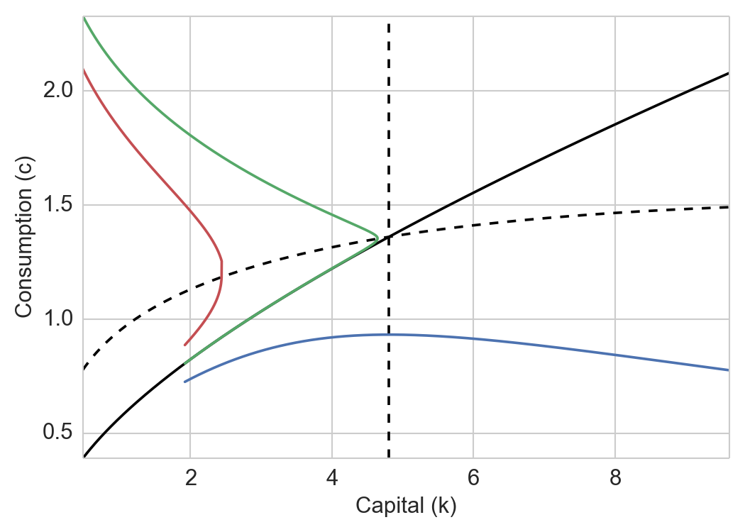
Depicted in is the state space over $(k,c)$. In solid black is the saddle path optimum function $c(k)$. The dotted lines delineate the various regions in terms of direction. To the left of the vertical dotted line (which is at $k^{\ast}$), consumption is increasing, and vice versa. Above the other dotted line, capital is decreasing, and vice versa. These can be computed from the laws of motion for each.

The lines in reg, green, and blue depict various candidate values for $c(0)$. The red line is above the saddle path and skews left into an infeasible region. The blue line is below the saddle path and falls towards zero consumption. The green path is exactly the saddle path choice. Notice that even here, tiny numerical errors prevent us from truly reaching the steady state. This isn't a huge problem as the computed value of $c(0)$ is nonetheless quite accurate, and we can re-update along the path.

Computation

There are two ways to do this: the easy way and the hard way. We can do a brute force discrete time approximation, or we can be a bit clever and get the same results with much less work. First the brute force method. We've already seen that the equilibrium is efficient, so let's just cut straight to solving the social planner's problem. For a given small time step $\Delta$ we have V(k) = \max_{i} \left\{\Delta u(f(k)-i)+\exp(-\Delta\rho) V(k+(i-\delta k)\Delta)\right\} An equivalent characterization would be choosing $k^{\prime}$ instead of $i$. Using the identity $k^{\prime} = k + \Delta i - \Delta\delta k$ we find V(k) = \max_{k^{\prime}} \left\{\Delta u(f(k)-(k^{\prime}-k)/\Delta-\delta k)+\exp(-\Delta\rho) V(k^{\prime})\right\} Thus by constructing a grid over capital and starting with an initial guess $V_0(\cdot)$, the above provides a method for updating our guess. Applying this mapping repeatedly until we reach a fixed point is called value function iteration. It can be slow, but it gets the job done.

Now on the the quicker method. The issue with choosing $c(0)$ to hit the steady state (the so called shooting method), as we saw in , is that even double precision floating point precision is not up to the task. There is one way around this: we can reverse time. Systems that are unstable in forward time are often stable in backwards time. By doing this and starting at a point perturbed infinitesimally from the steady state, and using negated laws of motion, we will actually trace out the saddle path.

Exogenous Growth Model

Let's consider only the simplest setting, in which the per-period utility function and production function are given by u(c) = \log(c) \qquad \text{and} \qquad f(A,k) = A k^{\alpha} This equilibrium will be efficient as before, so we'll cut straight to the social planner's problem. The value function can be expressed as \rho V = \max_{i} \left\{\log(Ak^\alpha-i)+(i-\delta k)V_k+gAV_A\right\} Let $\sim$ denote variables normalized by $z^{\frac{1}{1-\alpha}}$. In addition, consider the normalized value function $\tilde{V}$ characterized by V(A,k) = \tilde{V}\left(\frac{k}{A^{\frac{1}{1-\alpha}}},t\right) + \frac{1}{\rho}\left(\frac{1}{1-\alpha}\right)\left[\log(A)+\frac{g}{\rho}\right] From this we find V_k \align = A^{-\frac{1}{1-\alpha}} \tilde{V}_{\tilde{k}} \\ V_A \align = \frac{1}{A}\left(\frac{1}{1-\alpha}\right)\left(-\tilde{k} \tilde{V}_{\tilde{k}} + \frac{1}{\rho}\right) The reformulated value function equation is then \rho \tilde{V} = \max_{\tilde{i}}\left\{\log(\tilde{k}^{\alpha}-\tilde{i})+(\tilde{i}-\bar{\delta}\tilde{k})\tilde{V}_{\tilde{k}}\right\} where $\bar{\delta} = \delta + \frac{g}{1-\alpha}$. The analogous first order conditions is \frac{1}{\tilde{c}} = \tilde{V}_{\tilde{k}} and the envelope condition becomes (\rho+\bar{\delta}) \tilde{V}_{\tilde{k}} = \frac{\alpha \tilde{k}^{\alpha-1}}{\tilde{c}} + (\tilde{i}-\bar{\delta}\tilde{k})\tilde{V}_{\tilde{k}\tilde{k}} The normalized budget equation is $\tilde{y} = \tilde{c} + \tilde{i}$. Focusing on the steady state, we find the familiar expression \dot{\tilde{k}} = \tilde{i}-\bar{\delta}\tilde{k} = 0 Finally we arrive at an expression for the steady state normalized capital level \tilde{k}^{\ast} = \left[\frac{\alpha}{\rho+\bar{\delta}}\right]^{\frac{1}{1-\alpha}}

Outside of steady state, we can still make some headway. As before, define the function $m(t) = \tilde{V}_{\tilde{k}}(\tilde{k}(t))$, which is the value of the derivative along the optimum path. Consider the case of a known productivity path. Then we have \dot{m} = \dot{\tilde{k}} \tilde{V}_{\tilde{k}\tilde{k}} = (\tilde{i}-\bar{\delta}\tilde{k}) \tilde{V}_{\tilde{k}\tilde{k}} which leads to the characterization (\rho+\bar{\delta})m = \frac{\alpha \tilde{k}^{\alpha-1}}{\tilde{c}} + \dot{m} Thus the law of motion for the $(k,m)$ system is \dot{\tilde{k}} \align = \tilde{k}^{\alpha} - \bar{\delta}\tilde{k} - \frac{1}{m} \\ \dot{m} \align = -\left[\alpha\tilde{k}^{\alpha-1}-(\rho+\bar{\delta})\right] m Finally, expressing the above system in terms of $\tilde{c}$ and $\tilde{k}$ yields \dot{\tilde{k}} \align = \tilde{k}^{\alpha} - \bar{\delta}\tilde{k} - \tilde{c} \\ \dot{\tilde{c}} \align = \left[\alpha\tilde{k}^{\alpha-1} - (\rho+\bar{\delta})\right] \tilde{c} A very familiar expression. The only change really is that we are using $\bar{\delta}$ rather than $\delta$.